")
")


")


")

")
")
 in Excel & Google Sheets")


The easiest way to conditionally sum a column based on date ranges in Google Sheets is by using the SUMIFS or SUMPRODUCT functions. You can expand these formulas to sum values across multiple date ranges dynamically using the MAP and LAMBDA functions.
For example, you might want to sum transactions that fall between 01/02/2025 and 14/02/2025, or sum transactions within this period for a specific region. This can be easily accomplished using SUMIFS and SUMPRODUCT.
Sample Data
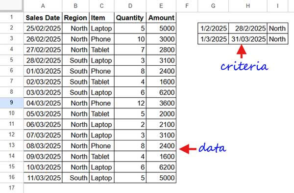
The criteria range is in G2:I3, where:
- Column G contains the start date
- Column H contains the end date
- Column I contains the region
Our goal is to find the total amount for each period (date range in G2:H2) for a specific region.
Array Formula to Conditionally Sum Date Ranges – Using SUMIFS
Let’s start with a basic non-array formula:
=SUMIFS($E$2:$E, ISBETWEEN($A$2:$A, G2, H2), TRUE, $B$2:$B, I2)Enter this formula in cell J2 and drag it down to J3 to apply it to the next criteria range.
Explanation:
E2:E: The range to sum (Amount column)ISBETWEEN(A2:A, G2, H2), TRUE: Returns TRUE if the date in A2:A falls between G2 and H2B2:B, I2: Filters by region
If you only need to sum based on date ranges (without filtering by region), remove $B$2:$B, I2 from the formula.
Convert to an Array Formula
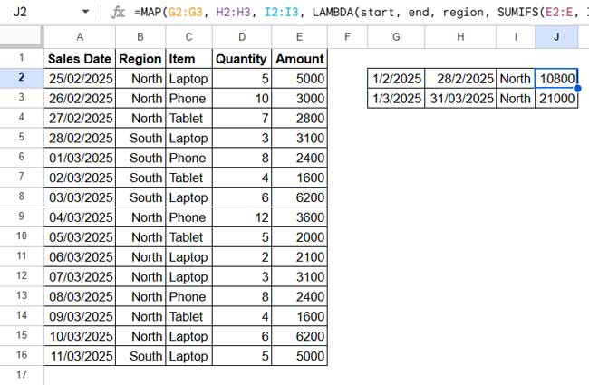
To apply this formula dynamically across multiple date ranges, use MAP + LAMBDA:
=MAP(G2:G3, H2:H3, I2:I3, LAMBDA(start, end, region, SUMIFS(E2:E, ISBETWEEN(A2:A, start, end), TRUE, B2:B, region)))If you don’t need to filter by region, remove I2:I3 from the MAP array, region from the LAMBDA parameters, and B2:B, region from the SUMIFS formula.
This formula dynamically sums values within each date range using an array formula, eliminating the need to drag the formula down manually.
Array Formula to Conditionally Sum Date Ranges – Using SUMPRODUCT
Another approach is using SUMPRODUCT.
Here’s the non-array formula:
=SUMPRODUCT($A$2:$A>=G2, $A$2:$A<=H2, $B$2:$B=I2, $E$2:$E)To remove the region condition, delete $B$2:$B=I2.
Convert to an Array Formula
To apply this across multiple date ranges, use MAP + LAMBDA:
=MAP(G2:G3, H2:H3, I2:I3, LAMBDA(start, end, region, SUMPRODUCT(A2:A>=start, A2:A<=end, B2:B=region, E2:E)))Both SUMIFS and SUMPRODUCT effectively conditionally sum date ranges.
Handling Trailing Zeros in Empty Rows
Both formulas return 0 in empty rows. To remove these, wrap the formula with an IF condition:
=ArrayFormula(IF(G2:G="", "", your_formula_here))This ensures that blank criteria rows don’t show 0, making the output cleaner.
Other Ways to Conditionally Sum Date Ranges in Google Sheets
While SUMIFS and SUMPRODUCT are the most common, you can also use QUERY or FILTER + SUM:
Using QUERY (SQL-Like Approach)
=QUERY(A1:E, "select SUM(E) where A >= date '"&TEXT(G2, "yyyy-mm-dd")&"' and A <= date '"&TEXT(H2, "yyyy-mm-dd")&"' and B='"&I2&"'")- Pros: Powerful and flexible.
- Cons: More complex.
Using FILTER + SUM
=SUM(FILTER(E2:E, ISBETWEEN(A2:A, G2, H2), B2:B=I2))- Pros: Simpler than QUERY.
- Cons: Requires SUM to be applied separately.
Conclusion
By using SUMIFS or SUMPRODUCT with MAP + LAMBDA, you can efficiently sum a column based on date ranges in Google Sheets. SUMIFS is more intuitive, while SUMPRODUCT offers a different approach. If you prefer an SQL-like method, QUERY is an alternative, and FILTER + SUM provides a compact solution.
Which method do you prefer? Let me know in the comments!
Resources
- Analyze Transactions by Date Range in Sheets: Start & End Dates
- Find the Date or Date Range from Week Number in Google Sheets
- COUNTIF to Count by Month in a Date Range in Google Sheets
- How to Include a Date Range in SUMIFS in Google Sheets
- How to VLOOKUP a Date Range in Google Sheets
- Filter Data by Date Range in Google Sheets
- Count Unique Dates in a Date Range – 5 Formula Options in Google Sheets
- Consecutive Dates to Date Ranges in Google Sheets: The REDUCE Method
Hi, I love this post so much, but I got an error when I tried it on my Sheet.
Can you give me a URL of a Google Sheet sample?
Hi, Hao Huynh,
The MMUL formula may not work if your data is large. But the SUMIFS would.
Please feel free to share the URL of your sample sheet below. I won’t publish it.