


XMATCH encompasses all MATCH functionalities in Excel, rendering MATCH unnecessary, except for compatibility with older Excel versions. Both functions are designed to retrieve the position of a value within a range.
This guide will explain the differences and similarities between XMATCH and MATCH using simple examples. We’ll compare them using two types of lists:
- One list with text, useful for explaining wildcard match.
- Three lists with dates, useful for illustrating the approximate match of the search key:
- One unsorted list.
- One sorted list from newest to oldest.
- One sorted list from oldest to newest.
XMATCH vs MATCH: Locating Text in Unsorted Range in Excel
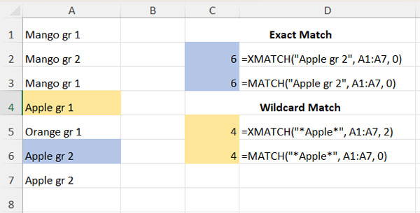
In the following examples, I have a list in Excel containing fruit names with grades in the range A1:A7. This is an unsorted list and values in the list occur more than once.
Let’s move on to a few examples.
Exact Match of Text
=XMATCH("Apple gr 2", A1:A7, 0) // returns 6
=MATCH("Apple gr 2", A1:A7, 0) // returns 6
Both formulas perform an exact match of the search key (lookup value) within the range, searching from the first value to the last value (top to bottom in vertical ranges and left to right in horizontal ranges).
In XMATCH, you can omit match mode 0 (zero), which represents the exact match, as it’s the default match mode.
However, in MATCH, you must specify 0, as the default match mode is 1.
Wildcard Match
=XMATCH("*Apple*", A1:A7, 2) // returns 4
=MATCH("*Apple*", A1:A7, 0) // returns 4
For a wildcard match, you must specify match mode 2 in XMATCH, but the match mode remains 0 in MATCH.
XMATCH vs MATCH: Locating Date or Number in Unsorted Range in Excel
In this comparison, we will use dates in the range A1:A6. When using dates as the search key, enter them in the syntax DATE(year, month, day).
Exact Match of Date
In numeric and date data types, the XMATCH and MATCH functions in Excel will work similarly to text criteria with respect to exact matches. Here are examples:
=MATCH(DATE(2024, 3, 15), A1:A6, 0) // returns 2
=XMATCH(DATE(2024, 3, 15), A1:A6, 0) // returns 2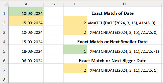
Wildcard Match
Wildcard matching is typically not applicable to date and number columns.
Exact Match or Next Smaller Date
Do not use the MATCH function with unsorted data for an approximate match in Excel, as it would return an incorrect result. Therefore, there is no scope for XMATCH vs MATCH comparison in this scenario.
=XMATCH(DATE(2024, 3, 11), A1:A6, -1) // returns 1This formula matches the date 11-03-2024 in the range, or if not available, it matches the next smaller date and returns the relative position.
Exact Match or Next Bigger Date
=XMATCH(DATE(2024, 3, 11), A1:A6, 1) // returns 2This formula matches the date 11-03-2024 in the range, or if not available, it matches the next bigger date and returns the relative position.
Here also, the XMATCH vs MATCH comparison is not applicable.
XMATCH vs MATCH: Locating Date or Number in Sorted Range
In sorted data, I won’t repeat the exact match, as it’s similar to unsorted data, and the wildcard match is not applicable. That being said, let’s proceed to formula examples.
Sorted Smallest to Largest (Ascending Order)
In a date or numeric range sorted in ascending order (smallest to largest value), we can use XMATCH and MATCH as follows:
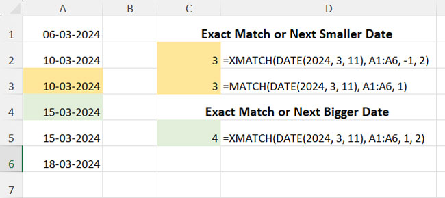
In the following formulas, the search key is the date 11-03-2024. The formulas exactly match the search key or match the next value that’s less than the search key.
=XMATCH(DATE(2024, 3, 11), A1:A6, -1, 2) // returns 3
=MATCH(DATE(2024, 3, 11), A1:A6, 1) // returns 3
The match mode (type) is -1 in XMATCH and 1 in MATCH. Additionally, we need to specify the search mode 2 (binary search) in XMATCH, which makes XMATCH faster compared to MATCH.
In XMATCH, additionally, you can specify match mode 1 for an exact match or the next value that’s greater than or equal to the search key.
=XMATCH(DATE(2024, 3, 11), A1:A6, 1, 2) // returns 4Sorted Largest to Smallest (Descending Order)
In a date or numeric range sorted in descending order (largest to smallest), we can use XMATCH and MATCH as follows:
=XMATCH(DATE(2024, 3, 11), A1:A6, 1, -2) // returns 3
=MATCH(DATE(2024, 3, 11), A1:A6, -1) // returns 3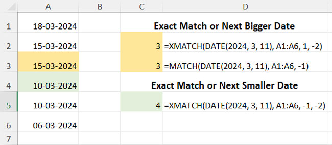
The match mode is 1 in XMATCH and -1 in MATCH, which is for an exact match of the search key or the next bigger value. We should specify binary search mode -2 in XMATCH.
In XMATCH, additionally, we can specify match mode -1 for an exact match or the next smaller value.
=XMATCH(DATE(2024, 3, 11), A1:A6, -1, -2) // returns 4Search from Last Value to First Value – The Powerful XMATCH Feature
In all the above examples, whether it is MATCH or XMATCH, the formulas perform the search from top to bottom in vertical ranges. If you specify a horizontal range, they will search from left to right.
In short, the formulas search from the first value to the last value. However, in XMATCH, you can specify searching from the last value to the first value, except in binary search mode.
What you need to do is specify search mode -1.
Syntax of XMATCH:
XMATCH(lookup_value, lookup_array, [match_mode], [search_mode])Syntax of MATCH:
MATCH(lookup_value, lookup_array, [match_type])Conclusion
In conclusion, while both MATCH and XMATCH serve the purpose of searching and matching values within Excel, XMATCH emerges as the preferred choice due to its wider array of search and match mode options. Especially in sorted data, XMATCH demonstrates superior performance.
Therefore, unless backward compatibility with older Excel versions is a concern, I recommend utilizing XMATCH over MATCH for its versatility and efficiency in various scenarios.
- Running Count of Occurrences in Excel (Includes Dynamic Array)
- Custom Sort in Excel (Using Command and Formula)
- Flip a Table Vertically in Excel (Includes Dynamic Array Formula)
- Running Total Array Formula in Excel [Formula Options]
- Address of the Last Non-Empty Cell Ignoring Blanks in a Column in Excel