


![Excel Hotel Room Availability Template [Free]](https://infoinspired.com/wp-content/uploads/2024/05/Excel-Hotel-Room-Availability-Template-218x150.jpg "Excel: Hotel Room Availability and Booking Template (Free)")


 in Google Sheets. For this, we can use the WHERE and OFFSET clauses)
By using the Query function, we can conditionally filter last n rows in a ‘data’ (range) in Google Sheets. For this purpose, we can use the WHERE and OFFSET clauses in the Query function in Sheets.
The WHERE clause enables us to apply the required condition to filter the data. Then with the help of the OFFSET clause, we can offset a ‘certain number’ of rows from the front to get the last N rows.
Actually, the purpose of the OFFSET in Query is to offset n number of rows. But we can use this clause dynamically to filter last n rows. Yes! That trick I am going to share with you in this post.
Before coming to the formula, let me tell you where this kind of filtering comes to use. I mean the real-life use of conditionally filtering last n rows in a dataset in Google Sheets.
Assume you have a list of teams and their score in the last 10 tournaments. To find the sum, average, max, and min of the last n results (scores) of a team, you can use my dynamic last n row filtering, which also conditionally.
A Similar Example:
Query Formula to Conditionally Filter Last N Rows in Google Sheets
As usual, let’s start with the sample data table. Just type the above values in columns B and C in your sheet.
Then type the filter condition/criterion in cell E2 and the last n rows that you want to filter in F2.
Done? Then let’s start to learn how to conditionally filter last n rows in Google Sheets.
Apply Condition Using WHERE in Query
Conditional filtering is just a child’s play if you know the use of Query. To master this, I suggest you read my following guide in your leisure time – Examples to the Use of Literals in Query in Google Sheets.
Also, find time to learn AND, OR, NOT in Query, Substring Match Using Contains, Like, Matches and Date Criteria Use in Query.
Here our task is just simple. In our topic, conditionally filtering last n rows, I am going to use only a single column, single condition filter.
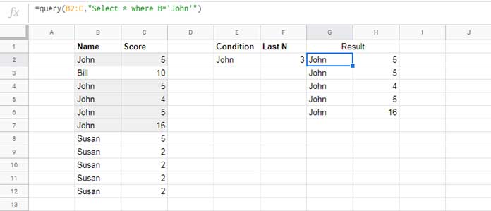
We just want to filter the data in the range B2:C, if the name in B2:B matches the criterion in cell E2, i.e. “John”.
Here is the required formula for that.
Criterion within formula;
=query(B2:C,"Select * where B='John'")
Criterion as cell reference;
=query(B2:C,"Select * where B='"&E2&"'")
Result:
COUNTIF in Query OFFSET to Filter Last N Rows in Google Sheets
We have completed the first part, i.e. conditionally filtering a dataset. Now we want to filter the last n rows from this output.
There is no clause in Query syntax to filter or conditionally filter last n rows in Google Sheets. We need to write a formula for that.
We can make use of the OFFSET clause in a certain way for this. The purpose of this clause is to offset a certain number of rows no matter whether the data is filtered or not.
To conditionally filter the last n rows, we can use the below logic.
=countif(B2:B,E2)Result: 5
The above COUNTIF will return the conditional count, which means the number of rows containing the criteria “John” in column B.
To find the number of rows to offset, use the above formula – n.
=countif(B2:B,E2)-F2If the value in F2 = 1, the above Countif formula would return 4. That means offset 4 rows and return the last 1 row.
The next question is how to connect the above Countif in Query. For that, we can follow the below approach.
We can use the just above Query formula as the data in another Query and offset the rows using the above Countif formula.
Conditionally Filter Last N Rows in Google Sheets – Syntax
=query(Query_formula,"Select * offset "&countif_formula)So here is the formula to conditionally filter last n rows in Google Sheets.
=query(query(B2:C,"Select * where B='"&E2&"'"),"Select * offset "&countif(B2:B,E2)-F2)Errors
The Query formula above would return #VALUE! error in two cases.
- When the filter condition is not available in the data range. I mean if the inner Query returns #N/A, the formula would return the said error.
- Last ‘n’ is greater the number of rows in the filtered output.
The formula would return #N/A! error, if the last ‘n’ is 0 or blank.
That’s all about how to conditionally filter last n rows using Query in Google Sheets.
Conditional SUM/AVERAGE/MAX/MIN Last N Results
Here are some real-life uses of the above type of last n row filtering. My following examples are based on the above data.
How to Sum Last N Values Conditionally in Google Sheets?
Formula:
=SUM(query(query(B2:C,"Select * where B='"&E2&"'"),"Select Col2 offset "&countif(B2:B,E2)-F2))How to Max/Min Last N Values Conditionally in Google Sheets?
Same as above. The only change here is the use of MAX/MIN instead of SUM.
Formula:
=MAX(query(query(B2:C,"Select * where B='"&E2&"'"),"Select Col2 offset "&countif(B2:B,E2)-F2))How to Average Last N Values Conditionally in Google Sheets?
For the conditional average of last n values, replace MAX with AVERAGE.
Formula:
=AVERAGE(query(query(B2:C,"Select * where B='"&E2&"'"),"Select Col2 offset "&countif(B2:B,E2)-F2))Additional Resources
- Find the Average of the Last N Values in Google Sheets.
- Address of the Last Non-Empty Cell Ignoring Blanks in Excel (Sheets also).
- How to Find the Last Row in Each Group in Google Sheets.
- How to Find the Last Matching Value in Google Sheets.
- Lookup Last Partial Occurrence in a List in Google Sheets.
- Lookup to Find the Last Occurrence of Multiple Criteria in Google Sheets.
- Vlookup Last Record in Each Group in Google Sheets.
- How to Find the Last Value in Each Row in Google Sheets.
- Consolidate Only the Last Row in Multiple Sheets in Google Sheets.
- Find the Last Non-Empty Column in a Row in Google Sheets.
- Count From First Non-Blank Cell to Last Non-Blank Cell in a Row in Google Sheets.