


This tutorial describes how to decode, or we can say, convert, a Unix Timestamp to local DateTime in Google Sheets.
In addition to the above how-to, I will explain how to convert a local DateTime to Unix time, I mean the reverse of the above.
I know most of you are familiar with or heard the terms Unix Time, Unix Timestamp, or Epoch Time. Actually, all these are referring to a 10-digit encoded UTC Date/DateTime.
Understanding Unix Time is essential to write a formula that converts Unix Timestamp to local DateTime or vice versa in Google Sheets.
I will try to explain about Unix Time in a nutshell even though you can Google it.
Unix Time is the seconds since 1st Jan 1970 (Epoch).
As you may know, a normal day (UTC) has a duration of 86400 seconds (24 hrs*60 minutes*60 seconds). These seconds play a vital role in the Unix Timestamp to local DateTime conversion formula in Google Sheets.
First, let’s go to the steps to convert a Local DateTime to Unix Time. That will help you better understand how to convert a Unix TimeStamp to local DateTime/Timestamp in Google Sheets.
Sheets Formula to Convert Local DateTime to Unix Time
To convert a local DateTime aka Timestamp to Unix Time, you can follow the below steps in Google Sheets.
Timestamp in Cell A2: 13/10/2019 09:54:00
To make you understand the conversion, before going to the formula, learn how to convert s Timestamp to Seconds in Google Sheets.
Timestamp to Seconds
See the formulas in cells C2 and C3 for the formula to convert DateTime aka Timestamp to seconds in Google Sheets.
I have used the Date and Time functions in these formulas.
| A | B | C | |
| 1 | DateTime | Number of Seconds | Formula |
| 2 | 01/01/1970 00:00:00 | 2209161600 | =DATE(1970,1,1)*86400 Which is equal to =A2*86400 |
| 3 | 13/10/2019 09:54:00 | 3780122040 | =(DATE(2019,10,13)+time(9,54,0))*86400 Which is equal to =A3*86400 |
You may think that subtracting the seconds, I mean B3-B2, will return the Unix Epoch Time of the DateTime in A3 since Unix Time is the number of seconds since Epoch (1/1/1970 00:00:00).
But, that’s only partially correct!
| A | B | C | |
| 4 | 1570960440 | =3780122040-2209161600 Which is equal to =B3-B2 |
To convert the local DateTime, we may need to include one more parameter. What’s that?
If the time in A3 is UTC, then the above =B3-B2 formula would convert the Timestamp to Unix Time. If not, you need to find the time zone (local time of your country) first.
In my case, it’s GMT+05:30. That means the time zone is five and a half hours ahead of UTC.
I must convert these five and a half hours to seconds. How?
| A | B | C | |
| 5 | 05:30 | 19800 | =time(5,30,0)*86400 Which is equal to =A5*86400 or =5.5/24*86400 |
Note:- Change 05:30 as per the time zone in your locale.
Unix Time Conversion from Local Datetime
We have now the GMT Offset in seconds in cell B5. As per the above example, we can convert the local DateTime to Unix Time as below.
=3780122040-2209161600-19800
Which is equal to;
=B3-B2-B5
or
=B4-B5
In simple terms, you can use the below formula to convert local DateTime to Unix Time in Google Sheets.
Generic Formula:
DateTime*86400-Epoch*86400-GMT*86400Note: If your timezone is GMT-, then use the Generic formula as;
DateTime*86400-Epoch*86400+GMT*86400In Short;
(DateTime-Epoch-GMT)*86400or
(DateTime-Epoch+GMT)*86400In the formula, as per my timezone, it would be like this:
=((DATE(2019,10,13)+time(9,54,0))-DATE(1970,1,1)-time(5,30,0))*86400Since our DateTime is in cell A3, we can replace the corresponding formula part (DATE(2019,10,13)+time(9,54,0) with the cell reference A3.
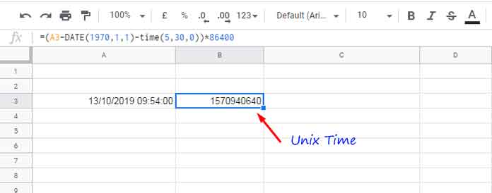
How to Convert Unix Timestamp to Local DateTime
Once you have learned the above conversion, the reverse of the same, I mean how to convert Unix Timestamp to local DateTime, is simple.
Here, our Unix Timestamp to convert to local DateTime is in cell B3.
First, convert that 10-digit Unix Time in seconds to a DateTime.
You can do that by dividing Unix Time by 86400.
1570940640/86400Then add Epoch Date Time and GMT to this DateTime.
=1570940640/86400+DATE(1970,1,1)+time(5,30,0)Please note that, if your timezone is GMT-, change the last part of the formula accordingly like -time(hr,min,sec).
In the final formula, you can replace Unix Time with the cell reference it contains, here cell B3.
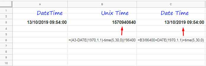
=B3/86400+DATE(1970,1,1)+time(5,30,0)In the following screenshot, you can see two formulas.
- Formula to convert local DateTime to Unix Time in cell B3.
- Formula to convert Unix Time to local Date Time in cell C3.
Update on 14-02-2023: Since we have the new EPOCHTODATE function, we can replace the C3 formula with =EPOCHTODATE(B3)+time(5,30,0).
I hope you could understand how to convert Unix Timestamp to local DateTime and vice versa in Google Sheets.
Related Reading:
- Convert Decimals to Minutes and Minutes to Decimals in Google Sheets.
- How to Add Hours, Minutes, Seconds to Time in Google Sheets.
- How to Increment Time By Minutes and Hours in Google Sheets.
- Round, Round-Up, Round Down Hour, Minute, Second in Google Sheets.
- Create a Countdown Timer Using Built-in Functions in Google Sheets.
- How to Convert Timestamp to Milliseconds in Google Sheets.
- How to Extract Date From Time Stamp in Google Sheets.