


In this tutorial, I am going to describe how to use the CUMPRINC function in Google Sheets. This is one of the financial functions available in Sheets.
The purpose of the CUMPRINC function in Google Sheets is to calculate the principal paid on a loan between a given period (a range of periods).
It’s important that the loan in question is based on constant-amount periodic payments and a constant interest rate.
The CUM in the CUMPRINC function stands for cumulative and PRINC stands for the principal. But the function for finding the principal of any given (single) period is PPMT, not PRINC. There is a reason for mentioning this here! What’s that?
To calculate the interest paid on a loan between a given period (a range of periods) is CUMIPMT and for any single period is IPMT.
Syntax and Arguments of the CUMPRINC Function in Google Sheets
Syntax:
CUMPRINC(rate, number_of_periods, present_value, first_period, last_period, end_or_beginning)Arguments: Please note there are no optional arguments in the CUMPRINC function in Google Sheets.
- rate – The interest rate.
- number_of_periods (Nper) – The total number of (count of) payments to be made.
- present_value (Pv) – The present value of the loan/annuity.
- start_period – The range starts with. Payment periods are numbered beginning with 1.
- If you want to calculate the cumulative principal for the period between 6 to 12, then your CUMPRINC start_period is 6.
- end_period – The range ends with.
- As per the start_period example above, it’s 12.
- Type – The timing of the payment, i.e. whether the payment is due at the end (0) or beginning (1).
For a 24 months loan, the start_period and the end_periond can be any number from 1 to 24. But the start period must always be less than or equal to the end_period.
Further, make sure you use consistent units for specifying rate and number_of_periods (Nper). To understand this, please first see the following input values for CUMPRINC formula in Google Sheets.
| A | B | |
| 1 | Loan Amount (Pv) | 25,000.00 |
| 2 | Rate (Annual Interest Rate) | 4.5% |
| 3 | Number_of_periods (Nper) in Years | 2 |
| 4 | First_period | 1 |
| 5 | Last_period | 24 |
| 6 | End_or_beginning | 0 |
This is a two-year loan and if you make monthly payments, you must use the interest 4.5%/12 in the formula as the rate and the Number_of_periods must be used as 2*12. Follow a similar approach in quarterly (divided by 4 and multiplied by 4) as well as in half-yearly (divided by 2 and multiplied by 2) payments.
CUMPRINC Formula Examples in Google Sheets
To calculate total principal for the 24 months period, use the CUMPRINC function as below.
=UMINUS(CUMPRINC(4.5%/12,2*12,25000,1,24,0))I have used the UMINUS additionally to change the sign of the cumulative principal from negative to positive.
Result: 250,000.00
I am rewriting the same formula using cell reference as the arguments.
=UMINUS(CUMPRINC(B2/12,B3*12,B1,B4,B5,B6))CUMPRINC Array Formula (Running PPMT Total in Google Sheets)
By feeding the CUMPRINC last_period with sequential numbers, you can generate the cumulative principal (running principal [PPMT] total) for all the periods.
The below Sequence formula returns the sequential numbers 1 to 24.
=sequence(24,1)Replace B5 in the earlier CUMPRINC formula with the above Sequence formula or the below Row formula.
=row(A1:A24)Then wrap the entire CUMPRINC formula with the ArrayFormula function.
=ArrayFormula(UMINUS(CUMPRINC(B2/12,B3*12,B1,B4,sequence(24,1),B6)))You can see the output of the above formula in column E on the below screenshot.
How to Calculate Cumulative Payment of a Loan in Google Sheets
Using the CUMPRINC and CUMIPMT functions you can calculate cumulative payment in Google Sheets.
Its actually like;
Cumulative Payment = CUMPRINC + CUMIPMTAssume the above CUMPRINC formula is in cell E2. Enter the following CUMIPMT formula in cell F2.
=ArrayFormula(UMINUS(CUMIPMT(B2/12,B3*12,B1,B4,sequence(24,1),B6)))Please note that here in the CUMIPMT, compared to CUMPRINC, all the parameters are the same except the function name.
The below formula in cell G2 will calculate the cumulative payment schedule of a 24-month loan in Google Sheets.
=ArrayFormula(E2:E25+F2:F25)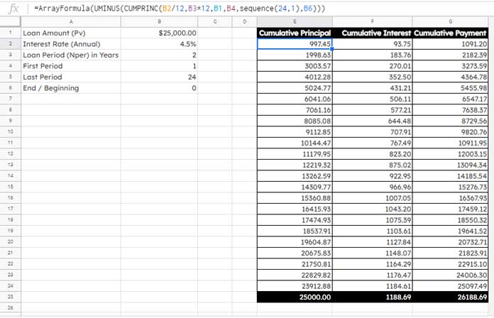
You May Like: Amortization Schedule in Google Sheets and Extra Principal Payments.
In the above-linked tutorial, I have shared a Google Spreadsheet containing an amortization schedule. See the tab “Sheet3” in that for the CUMPRINC function in live.
That’s all. Thanks for the stay, enjoy!