


![Excel Hotel Room Availability Template [Free]](https://infoinspired.com/wp-content/uploads/2024/05/Excel-Hotel-Room-Availability-Template-218x150.jpg "Excel: Hotel Room Availability and Booking Template (Free)")


In three-way lookup, there will be three search keys. Two from two columns and one from a row. To do a three-way lookup in Google Sheets, I am ‘only’ using the functions Vlookup and Match. Also, the use of the ampersand sign or Concatenate function is a must.
As a bonus I’ll try to provide you a three way lookup array formula too.
If I may use Index-Match, the popular three-way lookup solution among Excel users, I might not be able to generate a 3-way array lookup.
Here we go!
As an example, you can take a General Ledger (GL) Data (mock data) of a company.
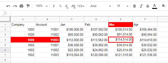
Lookup the company “1000” and Account “11003” in column A and B respectively (vertical Lookup). Then Lookup the month “Mar” in row # 1 (horizontal Lookup).
The end result would be the value $114,514.00 that available in the cell E4.
Non-Array Formula to Perform Three-way Lookup in Google Sheets
First, let me provide you the three-way lookup formula that works in Google Sheets. This formula may not expand (non-array) the results to additional rows/columns.
=ArrayFormula(vlookup(1000&11003,{A1:A&B1:B,C1:F},match("Mar",A1:F1,0)-1,0))This is similar to my two-way Lookup formula. The only change is in the use of the vertical Lookup search keys.
The search keys are combined using the ampersand as well as the columns A and B.
Google Sheets 3-way Lookup Formula Explanation
Some important points about the Google Sheets Vlookup function that can help you to change your mindset in the use of this trendy function.
The VLOOKUP is set to use the search key in the first column in the range. But there is flexibility in this.
For example, in the above GL data (range A1
The logic here is, combine the two search keys using the ampersand as well as the columns A and B in the GL data. So ultimately there will be one search key and one search column (no second column).
The combined search key:
1000&11003The combined columns in GL data:
{A1:A&B1:B,C1:F}Yes! Instead of A1:F we are using a virtual range as above. Now the third search key is “Mar” which is the month in row # 1.
What we want is to dynamcialy return the index column in Vlookup using the search key.
match("Mar",A1:F1,0)-1The above formula returns # 4. Actually, the column that contains the March month data is in column E, the fifth column.
Since I have combined the column A and B, the column number of column E in the above three-way lookup formula is 4 not, 5. The -1 in the above Match formula deals that.
This is the easiest formula to do a three-way Lookup in Google Sheets.
Array Formula for Three-way Lookup in Google Sheets
Multiple row output in 3-way Lookup is pretty easy if you could understand the above non-array 3-way Lookup formula.
I have highlighted the multiple column search keys, row search key (to find index number) and the outputs.
Formula:
=ArrayFormula(vlookup({1000&11003;1002&11002},{A1:A&B1:B,C1:F},match("Mar",A1:F1,0)-1,0))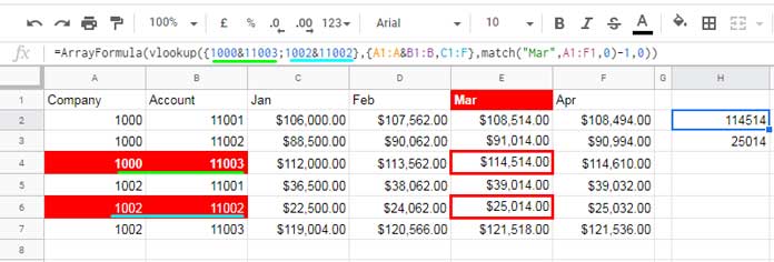
When you compare this formula with the non-array formula, you can understand that the change is in the search key usage.
See the underlined search keys in cyan and red color not only in the formula bar but also in the column A and B.
Finally I must explain how to take the criteria from cells.
Formula (in cell J2):
=ArrayFormula(vlookup(H2:H3&I2:I3,{A1:A&B1:B,C1:F},match(J1,A1:F1,0)-1,0))
That’s all. Hope you may share your thoughts on three-way Lookup in Google Sheets. Enjoy!
More Vlookup Resources:
- Vlookup from Bottom to Top in Google Docs Sheets.
- Vlookup Result Plus Next ‘n’ Rows in Google Sheets.
- Create Hyperlink to Vlookup Output Cell in Google Sheets.
- Vlookup Skips Hidden Rows in Google Sheets – Formula Example.
- How to Vlookup Importrange in Google Sheets [Formula Examples].
- Comparison of Vlookup Formula in Excel and Google Sheets.
- How to Vlookup a Date Range in Google Sheets [Sorted/Unsorted Data].
- How to Highlight Vlookup Result Value in Google Sheets.
As always, even on your busy day, you still managed to help me with my sheet with your advanced formula.
Thanks Prashant 😊
I’m happy to help.