We can use COUNTIF or COUNTIFS alongside an XLOOKUP formula to conditionally count the lookup results. This method functions similarly in both Excel and Google Sheets.

For instance, we can apply COUNTIF with XLOOKUP to retrieve a person’s attendance for a given month and count the times they were present or absent.

If we need to determine how many days they were present between a start date and an end date within a month, we can utilize COUNTIFS with XLOOKUP.

To perform lookups for multiple individuals, we can employ a Lambda function.

In this tutorial, we’ll explore these methods with straightforward examples. These solutions are applicable in Google Sheets and Excel versions supporting these functions, such as Excel 2021 and Excel in Microsoft 365.

Sample Data

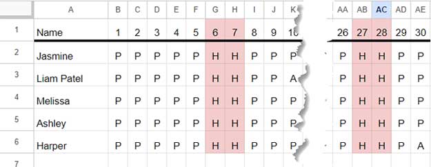
The sample data comprises the attendance records of 5 employees in cell range Sheet1!A1:AE6.

Employee names are listed in Sheet1!A2:A6, while their attendance is recorded in Sheet1!B2:AE6. In this attendance range, “P” denotes present, “A” denotes absent, and “H” denotes holiday.

Cells B1 through AE1 contain sequential numbers from 1 to 30, representing the 30 days of a calendar month.

In this tutorial, we’ll explore how to use both COUNTIF and COUNTIFS in conjunction with XLOOKUP within this range.

COUNTIF with XLOOKUP

Problem:

Retrieve the number of times an employee, whose name is entered in Sheet2!A1, is marked as present in the given table.

Formula:

=COUNTIF(XLOOKUP(A1, Sheet1!$A$2:$A$6, Sheet1!$B$2:$AE$6), "P")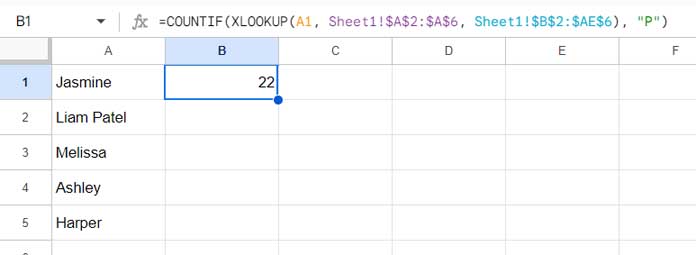

The COUNTIF function tallies the occurrences of “P” in the range XLOOKUP(A1, Sheet1!$A$2:$A$6, Sheet1!$B$2:$AE$6).

The formula adheres to the syntax COUNTIF(range, criterion):

• range: XLOOKUP(A1, Sheet1!$A$2:$A$6, Sheet1!$B$2:$AE$6)
• criterion: “P”

Understanding the range:

Examine the XLOOKUP function syntax: XLOOKUP(search_key, lookup_range, result_range, [missing_value], [match_mode], [search_mode]).

• search_key: A1
• lookup_range: Sheet1!$A$2:$A$6
• result_range: Sheet1!$B$2:$AE$6

XLOOKUP searches for the key in cell A1 within the range Sheet1!$A$2:$A$6 and returns the corresponding values from the identified row in Sheet1!$B$2:$AE$6.

Counting the Number of Present Instances for Multiple Employees

In the provided screenshot, the employee’s name in cell A1 is “Jasmine”, and the combined XLOOKUP and COUNTIF formula in cell B1 calculates her total number of present instances for the month.

Other employee names are listed down the column, specifically in cells A2 through A5.

To extend the calculation to other employees, you can drag the fill handle of cell B1 down.

However, if you prefer not to drag the formula down and want to use a lambda function, follow these steps:

Syntax: LAMBDA(parameter1, calculation)

In the lambda function, use a meaningful name, such as “employee”, for parameter1. The calculation will mirror the previous COUNTIF and XLOOKUP combo formula but substitute A1 with the parameter “employee”. The calculation becomes:

COUNTIF(XLOOKUP(employee, Sheet1!A2:A6, Sheet1!B2:AE6), "P")

Please make sure that you avoid spaces, cell references, or texts starting with numbers while naming references to prevent errors.

Now, incorporate this lambda function into the MAP function:

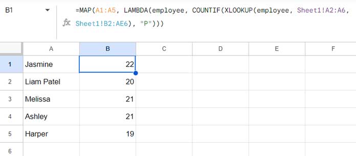
=MAP(A1:A5, LAMBDA(employee, COUNTIF(XLOOKUP(employee, Sheet1!A2:A6, Sheet1!B2:AE6), "P")))

Syntax: MAP(array1, lambda)

Where:

• array: A1:A5 (the range containing the employees)
• lambda: LAMBDA(employee, COUNTIF(XLOOKUP(employee, Sheet1!A2:A6, Sheet1!B2:AE6), "P"))

COUNTIFS with XLOOKUP

Problem:

Determine the frequency of instances where an employee, whose name is inputted in Sheet2!A1, is marked as present within the given table between days 10 and 20.

Formula:

=COUNTIFS(XLOOKUP(A1, Sheet1!$A$2:$A$6, Sheet1!$B$2:$AE$6), "P", Sheet1!$B$1:$AE$1, ">=10", Sheet1!$B$1:$AE$1, "<=20")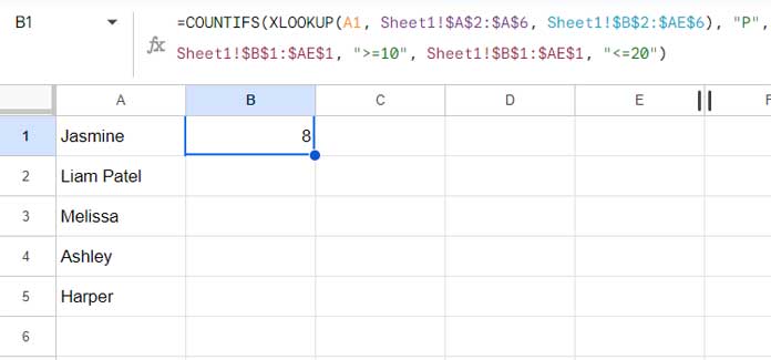

This formula calculates the number of days employee “Jasmine” was present between the 10th and the 20th.

This is an example of using COUNTIFS with XLOOKUP in Excel and Google Sheets.

In this formula, XLOOKUP’s role is to search for the name in cell A1 within the range Sheet1!$A$2:$A$6 and return the corresponding values from the found row in Sheet1!$B$2:$AE$6.

The COUNTIFS function then conditionally counts this range according to the following syntax: COUNTIFS(criteria_range1, criterion1, [criteria_range2, …], [criterion2, …])

Where:

• criteria_range1: Sheet1!$A$2:$A$6
• criterion1: “P”
• criteria_range2: Sheet1!$B$1:$AE$1
• criterion2: “>=10”
• criteria_range3: Sheet1!$B$1:$AE$1
• criterion3: “<=20”

To apply this calculation to other employees in cells A2:A5, you can either drag the B1 formula down or use the following MAP formula:

=MAP(A1:A5, LAMBDA(employee, COUNTIFS(XLOOKUP(employee, Sheet1!$A$2:$A$6, Sheet1!$B$2:$AE$6), "P", Sheet1!$B$1:$AE$1, ">=10", Sheet1!$B$1:$AE$1, "<=20")))

This formula is similar to our previous MAP formula that combined COUNTIF and XLOOKUP. The main difference lies in the calculation part within the lambda function. Here, a COUNTIFS and XLOOKUP combination is used, where “employee” replaces A1.

Conclusion

In the above examples, I’ve used Google Sheets function syntax to explain the formulas, and the screenshots are captured from Google Sheets.

While there may be slight differences in function parameters between Excel and Google Sheets, the core arguments remain the same. Therefore, the formulas presented above will function equally well in both applications.

This applies to all the formulas discussed, including those using COUNTIF with XLOOKUP, COUNTIFS with XLOOKUP, and the MAP function itself. No modifications are necessary for them to work seamlessly in either Excel or Google Sheets.