Function numbers are the function codes to use in subtotal aggregation in Google Sheets. They have many real-world uses, and they are a must-have when you deal with values in hidden cells.
Function numbers represent 11 of the most useful aggregation functions in Google Sheets, and you can use them to aggregate data presented in columns (vertical data), not rows.
This is certainly a drawback, but remember that we filter data in columns to filter out rows. In that sense, the vertical use of function codes is not a drawback.
At the time of writing this post, you can only use function numbers in Google Sheets in the SUBTOTAL function. However, in Excel, there is another function named AGGREGATE that also supports function numbers.
When should you replace your regular aggregation function with the SUBTOTAL + function number in Google Sheets?
There are three main instances when you might want to use function numbers in Google Sheets:
- When you want to omit hidden rows in the calculation range.
- When you want to place subtotals in a column.
- When you want to switch from one aggregation function to another function by calling a function number in a data validation drop-down.
The purpose of this tutorial is to provide you with the function numbers in Google Sheets. You can bookmark this page and check back when you want to use function codes in the SUBTOTAL function.
I’ll post all about SUBTOTAL in another tutorial.
Must Read: SUBTOTAL Function in Google Sheets: A Complete Guide
Google Sheets Aggregation Functions: Function Numbers and Use Cases
Eleven aggregation functions in Google Sheets have function number replacements. Each function has two function codes.
Here are the aggregation function names and their corresponding codes to use in SUBTOTAL.
| Function Name | Code I | Code II |
| AVERAGE | 1 | 101 |
| COUNT | 2 | 102 |
| COUNTA | 3 | 103 |
| MAX | 4 | 104 |
| MIN | 5 | 105 |
| PRODUCT | 6 | 106 |
| STDEV | 7 | 107 |
| STDEVP | 8 | 108 |
| SUM | 9 | 109 |
| VAR | 10 | 110 |
| VARP | 11 | 111 |
Can you give me a basic example?
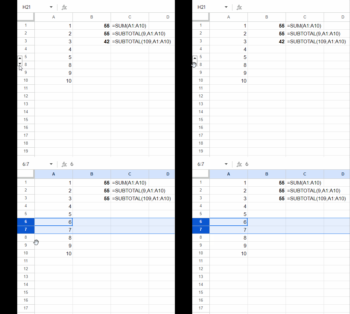
Sure. When you want to total the numbers in the range A1:A10, you usually use the following formula, right?
=SUM(A1:A10)You can replace that with the following SUBTOTAL formulas:
=SUBTOTAL(9,A1:A10)
=SUBTOTAL(109,A1:A10).
In the following screenshot, the formulas above are in cells B1, B2, and B3, respectively. See how the formula results change when I hide/unhide two rows.

How do the code I and code II sets of function numbers differ in function?
The code I set of function numbers excludes only cells hidden using the Data menu > Create a filter and Data menu > Add a slicer. The code II set of function numbers omits all types of hidden cell values.
Using Function Numbers in the SUBTOTAL Function in Google Sheets
Examples of Using All Function Numbers (Code II) in the SUBTOTAL Function in Google Sheets:
You can see below the 11 formulas and the results they return. Please note that the results are after hiding row 2 in the table.
Table #1 (Range A1:C5)
Table #1 contains three formulas that replace the AVERAGE, COUNT, and COUNTA functions.
| A | B | C | |
| Average | Count | CountA | |
| 1 | 50 | 50 | 50 |
| 2 | 50 | 50 | A |
| 3 | 50 | 50 | 50 |
=SUBTOTAL(101,A1:A3) // returns 50 | =SUBTOTAL(102,B1:B3) // returns 2 | =SUBTOTAL(103,C1:C3) // returns 2 |
Table #2 (Range D1:F5)
Table #2 contains three formulas that replace the MAX, MIN, and PRODUCT functions.
| D | E | F | |
| Max | Min | Product | |
| 1 | 70 | 70 | 50 |
| 2 | 60 | 60 | 50 |
| 3 | 50 | 50 | 50 |
=SUBTOTAL(104,D1:D3) // returns 70 | =SUBTOTAL(105,E1:E3) // returns 50 | =SUBTOTAL(106,F1:F3) // returns 2500 |
Table #3 (Range G1:I5)
Table #3 contains three formulas that replace the STDEV, STDEVP, and SUM functions.
| G | H | I | |
| Stdev | Stdevp | Sum | |
| 1 | 12 | 12 | 50 |
| 2 | 25 | 25 | 50 |
| 3 | 14 | 14 | 50 |
=SUBTOTAL(107,G1:G3) // returns 1.41 | =SUBTOTAL(108,H1:H3) // returns 1 | =SUBTOTAL(109,I1:I3) // returns 100 |
Table #4 (Range J1:K5)
Table #4 contains two formulas that replace the VAR and VARP functions.
| J | K | |
| Var | Varp | |
| 1 | 12 | 12 |
| 2 | 25 | 25 |
| 3 | 14 | 14 |
=SUBTOTAL(110,J1:J3) // returns 2 | =SUBTOTAL(111,K1:K3)// returns 1 |
Conclusion
If you use function numbers 1 to 11 instead of 100 to 111, you will get the same results if you hide row 2 using the Data menu > Create a filter or Data menu > Add a slicer.
However, if you hide row 2 by right-clicking on the row number and clicking Hide row, or by using Grouping, the results of using functions numbers 1 to 11 will be the same as the regular aggregation functions.
Here are some resources where you can see the use of the SUBTOTAL function.
- Subtotal with Condition in Google Sheets [Step by Step Guide]
- Find the Average of Visible Rows in Google Sheets
- Google Sheets Query Hidden Row Handling with Virtual Helper Column
- SUMIF Excluding Hidden Rows in Google Sheets [Without Helper Column]
- How to Omit Hidden or Filtered Out Values in Sum [Google Doc Spreadsheet
- COUNTIF | COUNTIFS Excluding Hidden Rows in Google Sheets
- Grouping and Subtotal in Google Sheets and Excel


