


")


")

")
")
 in Excel & Google Sheets")


To perform a VLOOKUP by date in a timestamp column in Google Sheets, we need to understand two key concepts. What are they?
1. Converting a Timestamp to a Date
A timestamp includes both the date and time, but we want to perform a VLOOKUP using only the date. This means we must convert the timestamp column to a date column before looking up values.
There are two functions that can help with this:
What is toDate?
It’s a scalar function in QUERY that we can use to extract only the date portion of a timestamp. This function ensures that VLOOKUP by date in a timestamp column works correctly.
2. Using the Modified Column in VLOOKUP
Once we’ve converted the timestamp column, we must ensure that it is correctly used in the VLOOKUP range along with the other relevant columns.
Didn’t get it? Let’s go through an example.
Example: VLOOKUP Issue with Timestamps
Assume we have a table with three columns: Timestamp, ID, and Amount (see Table #1 below).
| DateTime | ID | Amount |
| 25/08/2020 12:10:15 | KL601001 | 500 |
| 26/08/2020 13:00:10 | KL591050 | 500 |
| 27/08/2020 12:35:01 | KL604000 | 450 |
| 28/08/2020 11:49:00 | KL604002 | 0 |
| 29/08/2020 12:10:01 | KL592015 | 450 |
Our VLOOKUP search key is a date (e.g., 27/08/2020). Since column A contains timestamps, we must extract only the date before using it in VLOOKUP.
Method 1: Using QUERY with toDate
We modify the table virtually using QUERY, converting column A (timestamps) to dates.
Step 1: Creating the VLOOKUP Range
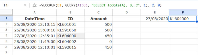
=QUERY(A1:C6, "SELECT toDate(A), B, C", 1)This formula:
- Extracts only the date from column A
- Keeps columns B and C unchanged
- Forms the correct VLOOKUP range
Step 2: Using VLOOKUP with the Modified Range
To return values from different columns based on the search key 27/08/2020 entered in cell E1:
- Fetch ID:
=VLOOKUP(E1, QUERY(A1:C6, "SELECT toDate(A), B, C", 1), 2, 0) - Fetch Amount:
=VLOOKUP(E1, QUERY(A1:C6, "SELECT toDate(A), B, C", 1), 3, 0) - Fetch both ID and Amount in one formula:
=ArrayFormula(VLOOKUP(E1, QUERY(A1:C6, "SELECT toDate(A), B, C", 1), {2, 3}, 0))
Note: If you are hardcoding the search key, use the DATE function instead of entering text:
=ArrayFormula(VLOOKUP(DATE(2020, 8, 27), QUERY(A1:C6, "SELECT toDate(A), B, C", 1), {2, 3}, 0))Method 2: Using INT Function
This is another efficient method for VLOOKUP by date in a timestamp column. The INT function removes the time portion, leaving only the date.
Step 1: Creating the VLOOKUP Range
={INT(A2:A6), B2:C6}This formula:
- Converts timestamps to dates using
INT - Retains columns B and C
Step 2: Using VLOOKUP with INT
=ArrayFormula(VLOOKUP(E1, {INT(A2:A6), B2:C6}, 2, 0))This returns KL604000, the ID corresponding to 27/08/2020.
VLOOKUP by Date in a Timestamp Column When the Timestamp Isn’t the First Column
What if the timestamp column isn’t the first column? Consider this shuffled table:
| ID | DateTime | Amount |
| KL601001 | 25/08/2020 12:10:15 | 500 |
| KL591050 | 26/08/2020 13:00:10 | 500 |
| KL604000 | 27/08/2020 12:35:01 | 450 |
| KL604002 | 28/08/2020 11:49:00 | 0 |
| KL592015 | 29/08/2020 12:10:01 | 450 |
Since the timestamp column is now the second column, we must adjust our QUERY and INT formulas.
Using QUERY
=QUERY(A1:C6, "SELECT toDate(B), A, C", 1)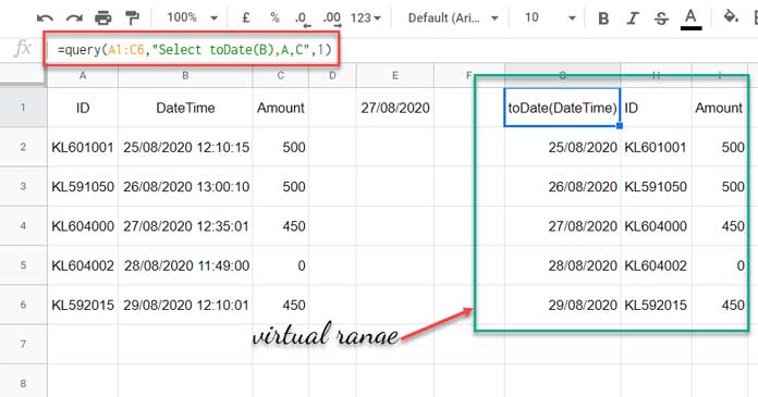
Using INT
={INT(B2:B6), A2:A6, C2:C6}The VLOOKUP formulas remain the same as before, but now reference column B instead of A.
Final Thoughts
Now you know how to perform VLOOKUP by date in a timestamp column in Google Sheets using two powerful methods: QUERY with toDate and the INT function.
Both methods ensure that VLOOKUP searches only dates, not full timestamps, allowing for accurate results.
Thanks for reading!
Resources
- How to VLOOKUP a Date Range in Google Sheets
- Extracting Date From Timestamp in Google Sheets: 5 Methods
- Comparing Timestamps and Standard Dates in Google Sheets
- How to Convert a Timestamp to Milliseconds in Google Sheets
- Convert Unix Timestamp to Local DateTime and Vice Versa in Google Sheets
- How to Use Timestamp within IF Logical Function in Google Sheets
- How to Unique Rows Ignoring Timestamp Column in Google Sheets
- How to Insert a Static Timestamp in Google Sheets
- How to Remove Milliseconds from Timestamps in Google Sheets