Mainly in two scenarios, you might want to use the UNIQUE and SUM functions together in Google Sheets:
- Unique values in a column and sum all values in another column, including duplicate rows.
- Sum the values of unique rows.
Do we exactly use the UNIQUE function and SUM function together here?
No. In the first case, we will use UNIQUE and SUMIF together, whereas in the second case, we will use UNIQUE, XLOOKUP, and SUM together.
Sample Data:
| Fruits | Qty. in Ton |
| Mango | 1 |
| Banana | 5 |
| Orange | 1.5 |
| Banana | 2.5 |
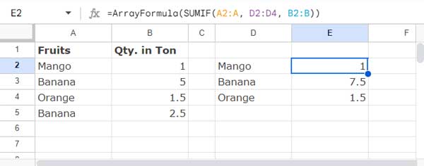
Our sample data consists of fruit names in column A and their quantities in column B. A1:B1 contains field labels, so we will use the A2:B range for the purpose.
Let’s find the unique fruit names and sum their quantities.
Scenario 1: Unique Values in One Column, Sum Values in Another
The first step is to extract the unique fruit names. For that, use the following formula in cell D2:
=UNIQUE(A2:A)To sum the values in column B that correspond to the unique values, use the following SUMIF formula in cell E2:
=ArrayFormula(SUMIF(A2:A, D2:D4, B2:B))
This follows the SUMIF syntax SUMIF(range, criterion, [sum_range]):
range:A2:Acriterion:D2:D4sum_range:B2:B
We use the ARRAYFORMULA since we have a criteria range, not a single criterion.
So, we have extracted unique values from column A and summed the corresponding values in column B using two formulas. We can combine these two and use them as a single entity using HSTACK.
Step 1:
In the SUMIF formula, replace the criterion D2:D4 with the UNIQUE formula.
=ArrayFormula(SUMIF(A2:A, UNIQUE(A2:A), B2:B))Note: We will modify this formula in each subsequent step.
Step 2:
Append the UNIQUE formula with the result from the previous step to generate a two-column table.
=HSTACK(
   UNIQUE(A2:A),
   ArrayFormula(SUMIF(A2:A, UNIQUE(A2:A), B2:B))
)
Step 3:
Use LET to name UNIQUE(A2:A) with a name such as uvs (unique values), and avoid repeating the formula twice.
=LET(
   uvs, UNIQUE(A2:A),
   HSTACK(
      uvs,
      ArrayFormula(SUMIF(A2:A, uvs, B2:B))
   )
)
Step 4:
Finally, use TOCOL with uvs to remove the empty cell at the last row of unique values.
=LET(
   uvs, TOCOL(UNIQUE(A2:A), 1),
   HSTACK(
      uvs,
      ArrayFormula(SUMIF(A2:A, uvs, B2:B))
   )
)
This way, you can use UNIQUE with SUM in Google Sheets.
Alternative Solution
The above method of using UNIQUE for one column and totaling another column can be replaced with a QUERY like this:
=QUERY(A1:B, "SELECT A, SUM(B) WHERE A <> '' GROUP BY A")Scenario 2: Sum Values of Unique Rows
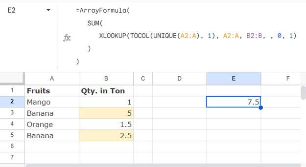
In our sample table, you can see that one item repeats twice, i.e., Banana. How do we total column B excluding the second occurrence of Banana?
In other words, how do we get the total of column B excluding duplicates in column A?
Formula:
=ArrayFormula(
   SUM(
      XLOOKUP(TOCOL(UNIQUE(A2:A), 1), A2:A, B2:B, , 0, 1)
   )
)
This follows the XLOOKUP syntax:
XLOOKUP(search_key, lookup_range, result_range, [missing_value], [match_mode], [search_mode])Where:
search_key:TOCOL(UNIQUE(A2:A), 1)(unique values in column A excluding blanks)lookup_range:A2:A(the range to look for the search keys)result_range:B2:B(the values to return for total)missing_value: omitted (the value to return when there is no match of search keys)match_mode:0(exact match of the search keys)search_mode:1(search from top to bottom)
The SUM function totals the values returned by XLOOKUP.
If you want to sum the values of the last occurrence, replace the search_mode 1 with -1.


Prashanth,
Can you help me? I am trying to get a dataset to sum only unique values for a certain date.
Date (A) | Weight (B)
2023-08-23 | 1487
2023-08-23 | 1487
2023-08-23 | 1487
2023-08-23 | 1487
2023-08-23 | 1462
2023-08-23 | 1462
2023-08-23 | 1462
2023-08-23 | 1462
2023-08-23 | 1431
2023-08-23 | 1431
2023-08-23 | 1431
2023-08-23 | 1431
The current formula is:
=SUMIFS(B:B, A:A, G2, B:B, UNIQUE(B:B))It sums the column by date when A:A is equal to G2 and B:B is unique. However, it keeps returning 0.
Hi Jessica Y,
You can use a combination of the SUM, UNIQUE, and FILTER functions as follows.
=SUM(UNIQUE(FILTER(B:B,A:A=G2)))Hi,
I’m facing an issue with three columns.
Here is a sample data set:
Name | Tickets | Department
Joe | 2 | Security
Tia | 3 | Reception
Joe | 4 | Security
Expected output:
Name | Tickets | Department
Joe | 6 | Security
Tia | 3 | Reception
I tried the Query you shared, and it works for 1 column and sum, but I am facing an issue in displaying multiple columns.
Any help is appreciated.
Thanks
– NS
Hi, NS,
You are on the right track. Use the QUERY() as below.
=query(A1:C,"Select A,sum(B),C where A is not null group by A,C label sum(B)'Tickets'",1)Thank you!
Prashanth,
I do have a question after all. I can’t figure out the formula when working with 3 columns of data, and I also need to ignore blank cells.
Example:
I want to unique sum column C based on columns A and B. I want to know how many jobs John Doe has Completed and the total amount for all completed jobs. I also want to ignore blank cells in column A. I also want to know how many jobs John Doe has “In Progress” and the total amount.
After that, I will use a simple
=query(A:A, "Order by DESC")for an employee ranking system.I am working with live data that auto-populates every 1min.
Hi, Frosty,
The following formula might help.
=query(A2:C,"Select A,count(C),sum(C) where A='John Doe' and B='Completed' group by A,B")Next, replace ‘Completed’ with ‘In Progress’
If you have any issue implementing the same, please feel free to share a sample Sheet (URL in your reply)
The following tutorial might help you progress in the popular QUERY function in Google Sheets.
What is the Correct Clause Order in Google Sheets Query?
Update:-
The following formula is for Unique and Sum every employee and to sort the sum column too.
=query(A2:C,"Select A,count(C),sum(C) where A is not null and B='Completed' group by A,B order by sum(C) desc,A asc")Prashanth! I can not thank you enough! It works and is precisely what I needed. You even took it a step further with the desc and asc! Thank you!
I do have one more question. The formula spits out count and sum text. Can I stop this or change the text the formula is producing?
Hi, Frosty,
You require to use the QUERY LABEL clause.
=query(A2:C,"Select A,count(C),sum(C) where A='John Doe' and B='Completed' group by A,B label count(C)'',sum(C)''")I hope that help.
I am working with live data that auto-populates. This formula is perfect, but I need it to ignore bank cells. Any chance it can do that?
Thank you,
-Scott
Never mind! I figured it out!
Hi, Frosty,
It’s nice to hear that you found a solution to it.
Even so, here are my suggestions for other users.
When using Query()
={unique(A2:A),ArrayFormula(sumif(A2:A,unique(A2:A),B2:B))}When using Sumif()
=ArrayFormula({unique(filter(A2:A,len(A2:A))),sumif(A2:A,unique(filter(A2:A,len(A2:A))),B2:B)})
Hi! I used your formula
={unique(A2:A5),ArrayFormula(sumif(A2:A5,unique(A2:A5),B2:B5))}successfully.I’m trying to alter the criteria a bit to look at unique information from A2:A5 + specific information from column B: B2:B5, “Y”.
I keep getting an error when trying to incorporate it into this formula. Are you able to help?
Hi, CT,
You may better use a QUERY.
Use the following formula when the group column is A, the criteria column is B, and the sum column is C.
=query(A2:C,"Select A,sum(C) where lower(B)='y' group by A label sum(C)''")Hi,
I used your formula (thank you!) for a list where there are some blanks.
Can you show me how to eliminate blanks from showing up in the array outcome?
={unique(D6:D35),ArrayFormula(sumif(D6:D35,unique(D6:D35),E6:E35))}Hi, matt,
Include Filter as below.
=ArrayFormula({unique(filter(D6:D35,len(D6:D35))),sumif(D6:D35,unique(filter(D6:D35,len(D6:D35))),E6:E35)})
Hi, thank you for this post.
I’m attempting to get the sum of unique values (Col B) that have “<2.5" (Col F) in the term "F1" (Col E).
I have this formula:
=SUMIFS(F:F,F:F,”< 2.5",E:E,"F1")And it gives the total of all grades with a Term of “F1” below 2.5.
Now, I need only to count each unique value 1x, to get the total number of students who have at least 1 grade below a 2.5 in “F1”.
Thank you.
Hi, Nathan Rayle,
I’m not clear about the last part of your query, i.e., “Now, I need…”
Can you share the URL of your Sheet (sample) in your reply below?
This is great! what’s the workaround if your original data does not match the same case? i.e., Banana or banana but I want them to show up as the same item count.
Hi, Danielle S,
Use UPPER or LOWER within QUERY()
When the range is A2:B5.
=query(A2:B5,"Select Upper(A), sum(B) group by Upper(A) label Upper(A)'',Sum(B)''")When you use an open range such as (A2:B).
=query(A2:B,"Select Upper(A), sum(B) where A is not null group by Upper(A) label Upper(A)'',Sum(B)''")Thank you for your time.
I have a job list that includes a lot of information per job, including wood types and colors used.
I have a list (without duplicates) using sort, unique, filter, and flatten functions.
I would like to add how many times each wood type and/or color is used.
Any help is appreciated.
Hi, Kris,
You may use Query().
If you share a sample, I will try to help you solve it. You can leave the address (Sheet URL) below.
Thanks so much for your help. Quick question, would you know if there is a way of using this Unique and Sumif array formula you’ve explained while sorting the numerical values from largest to smallest?
Kind regards,
Mr. A
Hi, Mr. A,
Include SORT as below.
=SORT({unique(A2:A5),sumif(A2:A5,unique(A2:A5),B2:B5)},2,0)Note:- Removed the ArrayFormula as the SORT takes care of the role.
I am trying to get a total of one column and only including the unique entries from another column. I am getting an error message stating formula parse error.
This is the formula I am using.
={unique(D5:D800), ArrayFormula(sumif(D5:D800, unique(D5:D800), K5:K800)}What do I need to do to correct this?
Hi, Janice Lane,
Try this instead. You were missing one closing bracket before the last curly bracket.
={unique(D5:D800), ArrayFormula(sumif(D5:D800, unique(D5:D800), K5:K800))}This is great, can I ask how I would bring the first column and the total entries for each? I am trying to get UNIQUE and COUNTIF to work together.
Hi, Norman Navarro,
You may simply try the below Query.
=query(A1:A,"Select A,count(A) where A is not null group by A",1)If the range A1:A doesn’t have the header row (label in A1), then use 0 instead of 1 in the last part of the above Query.
I am trying to do exactly this, but only return the sums without the first column:
I got
{ArrayFormula(sumif(ExpensesDB!A2:A,unique(ExpensesDB!A2:A),ExpensesDB!C2:C))}but this didn’t combine all of the common month numbers it just returned everything from Column A.Hi, Nick,
You can try this.
={unique(ExpensesDB!A2:A),ArrayFormula(sumif(ExpensesDB!A2:A,unique(ExpensesDB!A2:A),
ExpensesDB!C2:C))}
Here is another tutorial in line with the above.
Sum by Month in Google Sheets Using Combined SUMIF Formula
I am trying to create this arrangement but bringing the information from a second sheet ( in the same file) but does not work this formula.
Do you know why?
Please share an example sheet.