")
")


")


")

")
")
 in Excel & Google Sheets")


You usually use Format > Number > Percent to format a number as a percentage in Google Sheets. If you wish to do that with a function instead, you can use the TO_PERCENT function in Google Sheets.
The function has an edge over the format menu command. When you use the format menu, you need to apply it to a specific cell or cell range. On the contrary, the formula helps you get the result directly in the formula-applied cell or at the offset you specify inside the formula.
We’ll see that with examples below. Before we go into that, let’s proceed to the syntax part.
Syntax of the TO_PERCENT Function in Google Sheets
Syntax:
TO_PERCENT(value)Argument:
- value – The number or reference to a cell to format as a percentage.
If the value is a text or an error, the function will retain the value/error.
If it’s a date or time, it will format it as a percentage — which, of course, may not be meaningful.
Examples of the TO_PERCENT Function in Google Sheets
Imagine a student scored 525 marks out of 600 on a test.
In A1, you would enter:
=525/600This gives 0.875 in A1.
Then in B1, you can show it as a percentage:
=TO_PERCENT(A1)This displays 88% in B1.
If you don’t use the TO_PERCENT function, you could directly format cell A1 manually via Format > Number > Percent.
The Advantage of Using TO_PERCENT over Manual Formatting
The benefit of using TO_PERCENT is its dynamic behavior. You don’t need to stick with any particular cell.
For example, when you dynamically insert a total row into a filtered table, the number of rows in the result may update. So you don’t know the exact cell to manually format. Here, you can use the TO_PERCENT function to handle it automatically.
Example
Assume you have student names in column A, subjects in column B, and marks in column C. The student names appear three times, as each student has attended three papers. Each test is out of 100 marks.
| Name | Subject | Marks |
| Ben | Physics | 88 |
| Ben | Chemistry | 90 |
| Ben | Maths | 100 |
| Mike | Physics | 99 |
| Mike | Chemistry | 99 |
| Mike | Maths | 99 |
| Leo | Physics | 79 |
| Leo | Chemistry | 88 |
| Leo | Maths | 96 |
The following formula in E2 would return the data related to Ben along with the percentage of total marks scored:
=VSTACK(
   FILTER(A2:C, A2:A="Ben"),
   HSTACK("Total Percentage (out of 300)", , TO_PERCENT(SUM(FILTER(C2:C, A2:A="Ben"))/300))
)
Resulting Table:
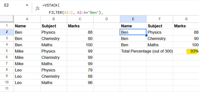
The benefit of this formula is that you can cut and paste it to a different cell, and the marks will retain their numeric formatting while the total will remain properly formatted as a percentage using TO_PERCENT.
Note
When using the TO_PERCENT function in Google Sheets, ensure the cell is formatted as Format > Number > Automatic. If the cell is pre-formatted using Format > Number with any other format, the result of the TO_PERCENT function will not display as a percentage but will instead follow the pre-existing formatting. To avoid this issue, make sure the cell is set to Automatic formatting before applying the function.
Resources
- Fix Fractional Percentage Formatting Issues in Google Sheets
- How to Calculate Percentage Difference in Google Sheets
- How to Calculate Reverse Percentage in Google Sheets
- How to Calculate Percentage of Total in Google Sheets
- How to Round Percentage Values in Google Sheets
- Percentage Change Array Formula in Google Sheets