Tick Boxes can help you organize your data in various ways. You can use Tick (✓) Boxes to indicate the status of activities in a list. Below, you’ll find 10 useful Tick Box tips and tricks in Google Sheets that I’ve come across. I hope you find them helpful!

The Tick Box in Google Sheets is interactive. When checked, it indicates TRUE, meaning “Yes,” the activity is completed or the answer is correct. By default, it is FALSE.

10 Must-Learn Tick Box Tips and Tricks in Google Sheets

Here are my 10 useful Tick Box tips and tricks in Google Sheets for all the passionate Google Sheets users out there. Some of these tips are explained in detail in my earlier posts. In those cases, I’ll provide a brief description here and include links to the full tutorials in the ‘Resources’ section at the bottom.

1. Insert Tick Boxes in Google Sheets

It’s straightforward. Select the cells where you want to insert Tick Boxes. Then, go to the menu Insert and click on Tick box. That’s all you need to do to insert interactive Tick Boxes.

2. Count Checked and Unchecked Cells

It’s simple. Suppose you have several Tick Boxes in the range A1:A. Use the following COUNTIF formula to count the checked boxes:

=COUNTIF(A1:A, TRUE)

Change TRUE to FALSE in this formula to count the unchecked boxes.

3. Conditionally Change the Tick Box Color

From my list of the best Tick Box tips and tricks in Google Sheets, this conditional formatting trick is my favorite.

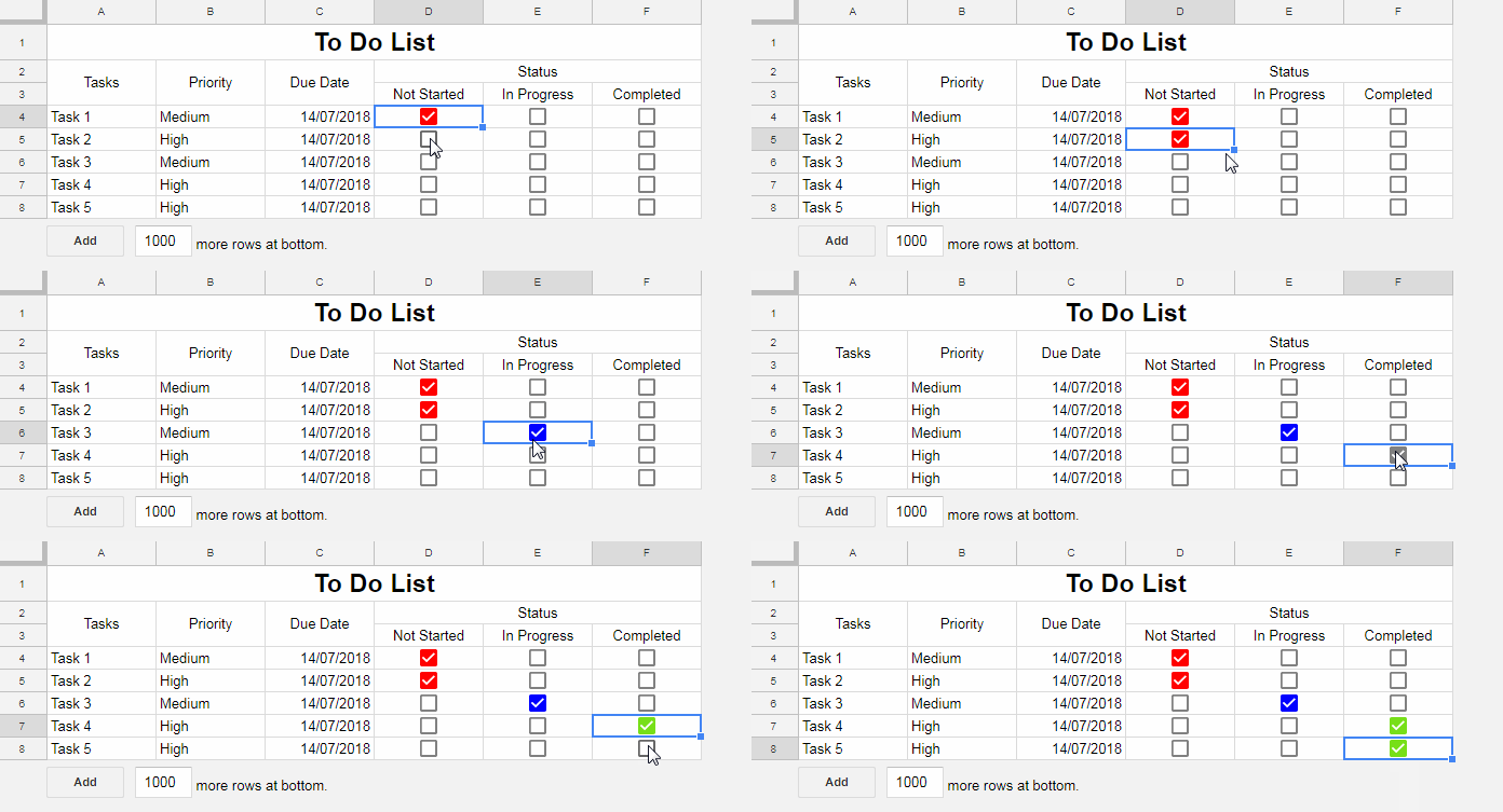
By default, the color of a Tick Box is dark grey. You can change its color easily using conditional formatting.

Although the Tick Box is technically a character, and you can change its color like any font, this method lets you selectively change the color of checked Tick Boxes. Let’s see how to do it:

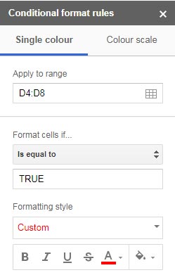
1. Select the cells with the Tick Boxes. For example, select the range D4:D8.
2. Go to the menu: Format > Conditional formatting.
3. Under Format rules, choose Is equal to and type TRUE.
4. In the Formatting style section, choose the font color you want for checked Tick Boxes and set the fill color to None.

Click Done, and the checked Tick Boxes will now appear in your chosen color.

You can apply this method to other ranges, such as E4:E8 or F4:F8, to customize their colors as well.

4. Extract Rows Containing Checked Tick Boxes

If you have a list of student names in column A and Tick Boxes in column B, you can extract rows with checked Tick Boxes using these formulas:

• Using QUERY:

=QUERY(A1:B, "SELECT * WHERE B=TRUE")

• Using FILTER:

=FILTER(A1:B, B1:B)

5. Create Dynamic Charts by Controlling Chart Data Using Tick Boxes in Google Sheets

This is my second favorite tip among the 10 Tick Box tips and tricks in Google Sheets.

When reporting project status to a client on a weekly, fortnightly, or monthly basis, you can rely on a Combo Chart. Combo charts in Google Sheets are useful for tracking job progress against a schedule.

Understanding the Data

Here’s a sample project schedule showing its progress and completion status. The project was scheduled for 5 weeks but was completed in 6 weeks.

Sample Sheet

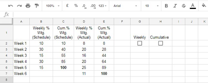
Chart Data Breakdown:

• Column A: Weekly schedule, showing the allowed weeks (5) and the extra week required for completion (6).
• Column B: Total % Weightage of tasks planned, summing up to 100%.
• Column C: Cumulative planned % Weightage.
• Column D: Actual % Weightage of completed tasks.
• Column E: Cumulative actual % Weightage.

What is % Weightage?

The total % Weightage of a project is 100. This value is distributed among individual tasks based on factors like time, manpower, and cost. Each week’s tasks are summed to give the weekly Weightage in Column B, while Column D shows actual completion progress.

The Role of Tick Boxes

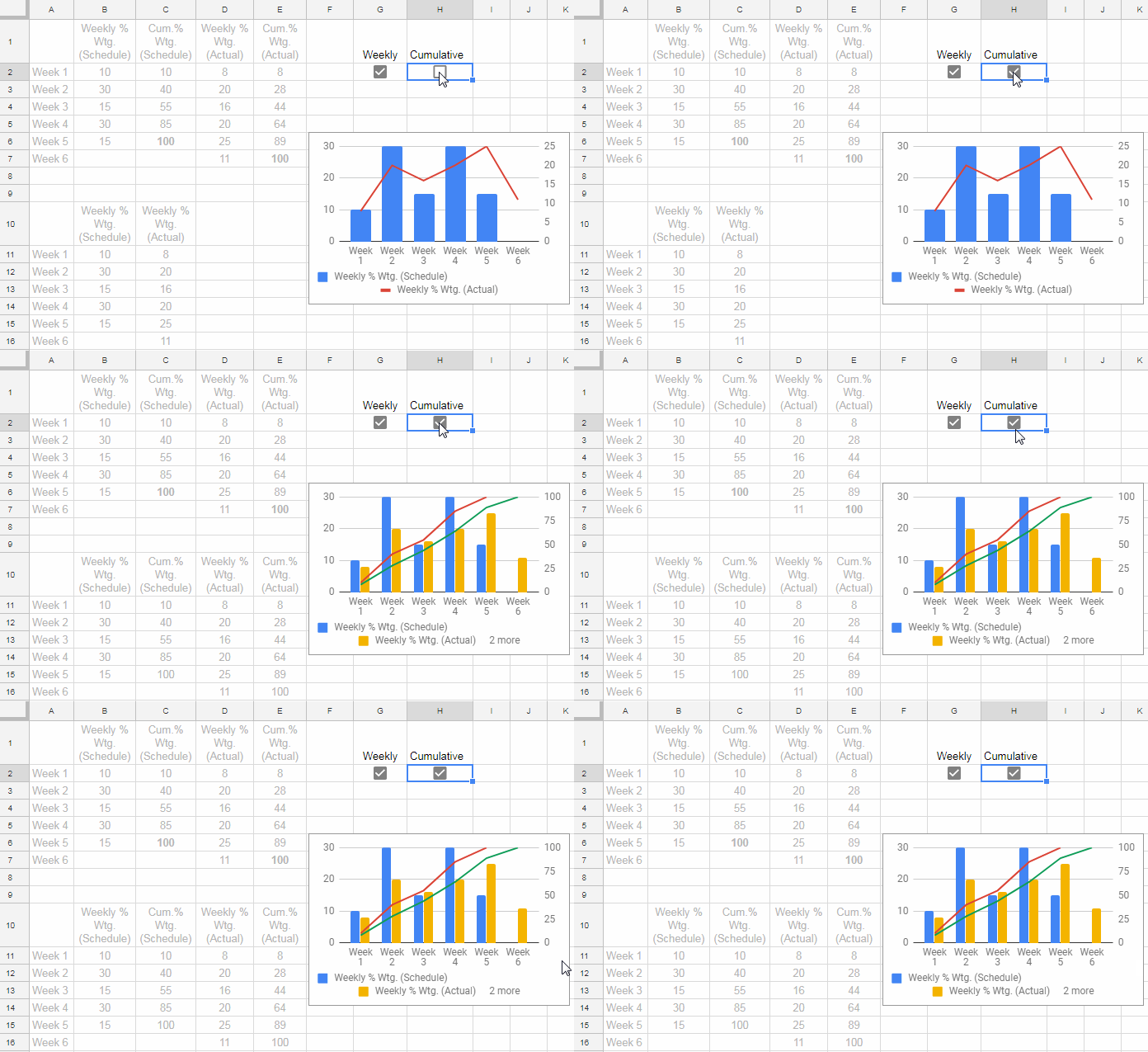
Tick Boxes in cells G2 and H2 control the data displayed in the chart. Here’s the formula in cell A10 that dynamically extracts data:

=IF(
   AND(G2=TRUE, H2=TRUE), {A1:E7}, 
   IF(
      AND(G2=TRUE, H2=FALSE), {A1:B7, D1:D7}, 
      IF(
         AND(G2=FALSE, H2=TRUE), {A1:A7, C1:C7, E1:E7}
      )
   )
)

Formula Explanation:

• If both Tick Boxes are checked, the formula extracts the full data range (A1:E7).
• If only the first Tick Box is checked, it extracts weekly data (A1:B7 and D1:D7).
• If only the second Tick Box is checked, it extracts cumulative data (A1:A7, C1:C7, and E1:E7).

Creating a Dynamic Combo Chart with Tick Box Control

To create the chart:

1. Select the data range A10:E16.
2. Go to Insert > Chart.
3. In the Chart editor, configure the following:
   • Under Setup Tab:
     • Chart type: Combo Chart
     • Stacking: None
   • Under Customize Tab:
     • For series starting with “Cum”:
       • Type: Line
       • Axis: Right
     • For series starting with “Weekly”:
       • Type: Column
       • Axis: Left

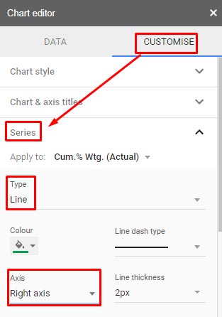
Now your dynamic combo chart is ready! Use the Tick Boxes to control the displayed chart series easily.

6. Retain Tick Boxes with Imported Data

Just like any text, you can copy and paste Tick Boxes into different cells. However, if you use a formula to copy a Tick Box, you won’t get the Tick Box itself. Instead, you’ll only get its value: TRUE (checked) or FALSE (unchecked).

For instance, if you have a Tick Box in cell A1 and reference it in B1 using the formula =A1, cell B1 will display either TRUE or FALSE depending on the state of the Tick Box in A1.

This issue also occurs when you use functions like IMPORTRANGE, FILTER, or QUERY to import or process data containing Tick Boxes.

To overcome this and display a Tick Box-like character instead of TRUE or FALSE, follow these steps:

Example: Creating Custom Tick Box Characters

1. Select the range A1:A10.
2. Go to Data > Data validation.
3. Click Add Rule.
4. Under Criteria, select Tick box and check Use custom cell values.
5. Enter the following custom characters:
   • Unticked: ☐
   • Ticked: ☑
6. Click Done.

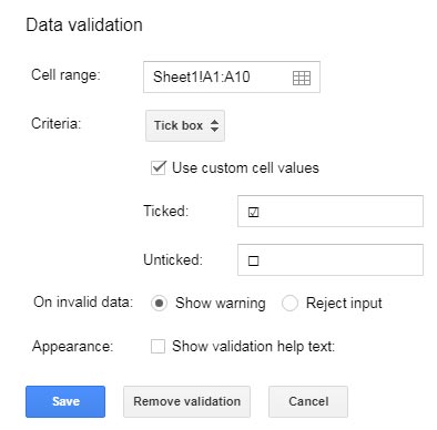
Now, instead of displaying TRUE or FALSE, the formula results will show the custom characters ☐ (for unchecked) and ☑ (for checked).

Alternative Method: You can also select the cells with TRUE/FALSE values and go to Insert > Tick box to reinsert Tick Boxes in the new location.

7. Select or Deselect Multiple Tick Boxes at Once

You can quickly select or deselect multiple Tick Boxes by selecting the range and pressing the spacebar.

8. Use Tick Boxes in To-Do Lists

Here’s how to apply a strike-through effect to mark completed tasks using Tick Boxes in a to-do list.

For example, in the following to-do list, the data range is A4:D8:

• Column A: Tasks
• Column B: Priority
• Column C: Due Date
• Column D: Status (contains Tick Boxes)

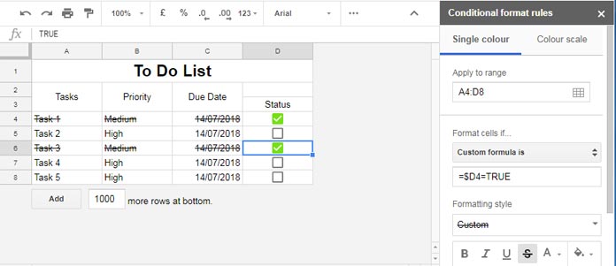
When you tick a box in Column D, you want the corresponding row to be struck through.

Follow these steps:

1. Select the range A4:C8.
2. Go to Format > Conditional formatting.
3. Under Format rules, select Custom formula is.
4. Enter the formula: =$D4=TRUE
5. Under Formatting style, select Strikethrough and set the Fill color to None.
6. Click Done.

Now, when you check a Tick Box in Column D, Google Sheets will automatically strike through the content in the corresponding row (A4:C8).

9. Highlight Rows Based on Tick Box Selection

To highlight a row when a Tick Box is checked, follow the same steps as in the strike-through example.

Instead of selecting Strikethrough under Formatting style, choose a Fill color of your choice.

10. Delete Tick Boxes in Google Sheets

To delete a Tick Box, select the cell and press the Delete key. Alternatively, go to Edit > Delete > Values.

Resources

Here are some related tutorials you might find useful:

• Assign Values to Tick Boxes and Calculate Totals in Google Sheets
• Change Tick Box Color While Toggling in Google Sheets
• Check/Uncheck Tick Boxes Based on Another Cell’s Value
• Highlight Multiple Groups Using Tick Boxes in Google Sheets