In this tutorial, I’ll show you whether we can use SUMIF across multiple Sheets in Google Sheets, or if not, what the best alternative is.

The SUMIF function works well when applied to a single range within a Sheet.

If you want to use it across multiple ranges—whether within the same Sheet or from several Sheets—you should first append those ranges vertically into one Sheet.

You can use the VSTACK function to do that. Here’s its syntax:

VSTACK(range1, [range2, …])

Once appended, you’ll have a new physical range where you can apply the SUMIF conditional sum.

Without a physical range, the function will return the infamous “Argument must be a range” error. Here’s an example of that issue:

=SUMIF(
  VSTACK('April 23'!B2:B10,'May 23'!B2:B11),
  "Stationery",
  VSTACK('April 23'!C2:C10,'May 23'!C2:C11)
)

The above is an attempt to use SUMIF across two Sheets. However, it returns #N/A because the input is not recognized as a proper range.

So that leaves us with two valid options when you want to SUMIF across multiple Sheets in Google Sheets:

1. Append the ranges to a new Sheet in the same workbook, and use SUMIF on that physical range.
2. Use the formula for appending ranges directly inside a QUERY function.

We’ll see examples of both approaches below.

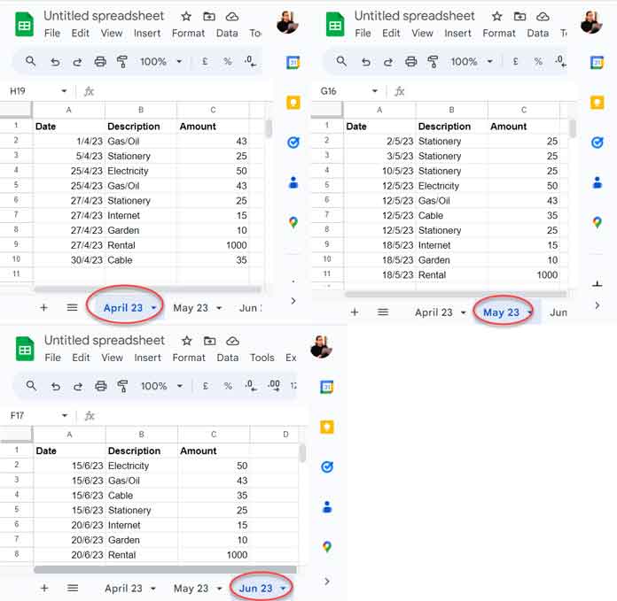
Sample Data: Daily Expense Sheets

Assume my daily expense data is spread across multiple Sheets in a workbook, and “Internet” is one of the expense categories.

The daily entries are stored in three Sheets: “April 23,” “May 23,” and “Jun 23.”

Copy the Sample Sheet

We’ll now learn how to SUMIF across multiple Sheets in Google Sheets to total the expense on the item “Internet.”

Append Ranges Across Sheets Vertically for SUMIF

We want to apply SUMIF across the ranges A1:C in Sheets “April 23,” “May 23,” and “Jun 23.”

The field labels are: Date, Description, and Amount in cells A1:C1 (as shown in the screenshot above).

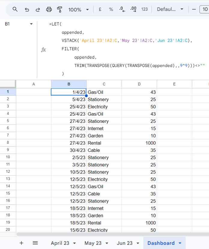
With the help of VSTACK, we can append the ranges A2:C vertically from these Sheets into a fourth Sheet named “Dashboard.”

We use A2:C instead of A1:C to exclude the header row in each Sheet.

Formula (Dashboard!B1):

=LET(
  appended,
  VSTACK('April 23'!A2:C, 'May 23'!A2:C, 'Jun 23'!A2:C),
  FILTER(
    appended,
    TRIM(TRANSPOSE(QUERY(TRANSPOSE(appended),,9^9)))<>""
  )
)

Note:

The VSTACK is sufficient to create the combined range. However, there could be hundreds of blank rows between ranges. The FILTER formula removes those empty rows.

Related: Filter Out If the Entire Row Is Blank in Google Sheets

Now we’re ready to use SUMIF across multiple Sheets in Google Sheets.

But first, you might ask:

“Can I refer to the Sheet names listed in a range (like A1:A) instead of hardcoding them into the VSTACK formula?”

Yes, you can! Use the following formula in Dashboard!B1:

=LET(
  data,
  REDUCE(TOCOL(,1), TOCOL(A1:A, 1), LAMBDA(a, v, IFERROR(VSTACK(a, INDIRECT(v&"!A2:C"))))),
  FILTER(data, TRIM(TRANSPOSE(QUERY(TRANSPOSE(data),,9^9)))<>"")
)

Here, A2:C is the range to append, and A1:A contains the Sheet names.

Important:

• When entering Sheet names like “April 23,” Google Sheets might treat them as dates. So select A1:A, then go to Format > Number > Plain text before entering the names.
• The date values in column B of the combined data may show as date values. Select the column and format it using Format > Number > Date.

If the formula is too complex, you can also use my custom named function: COPY_TO_MASTER_SHEET.

SUMIF Across Multiple Sheets in Google Sheets

Syntax: SUMIF(range, criterion, [sum_range])

Now, let’s use SUMIF across multiple Sheets in Google Sheets to total the expense for “Internet.” It’s as simple as:

=SUMIF(Dashboard!C1:C, "Internet", Dashboard!D1:D)

To make the formula dynamic, place the criterion in E1 and use:

=SUMIF(Dashboard!C1:C, E1, Dashboard!D1:D)

What if you want to use multiple criteria?

Let’s say you want to sum expenses for “Cable” and “Internet”:

=ArrayFormula(SUMIF(Dashboard!C1:C, E1:E2, Dashboard!D1:D))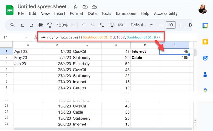

Hardcoded version:

=ArrayFormula(SUMIF(Dashboard!C1:C, VSTACK("Internet", "Cable"), Dashboard!D1:D))

Skipping the “Dashboard” Helper Sheet

Not everyone likes to create an extra helper Sheet (like “Dashboard”) just for appending data.

If that’s you, use this QUERY alternative instead of SUMIF across multiple Sheets in Google Sheets:

Replace append_formula with the same formula used in Dashboard!B1.

=QUERY(append_formula, "SELECT Col2, SUM(Col3) WHERE LOWER(Col2) = 'internet' GROUP BY Col2 LABEL SUM(Col3)''", 0)

The condition is case-sensitive, so “Internet” must be written in lowercase.

To use a dynamic cell like E1:

=QUERY(append_formula, "SELECT Col2, SUM(Col3) WHERE LOWER(Col2) = '"&LOWER(E1)&"' GROUP BY Col2 LABEL SUM(Col3)''", 0)

For multiple values like “Cable” and “Internet”:

=QUERY(append_formula, "SELECT Col2, SUM(Col3) WHERE LOWER(Col2) MATCHES 'cable|internet' GROUP BY Col2 LABEL SUM(Col3)''", 0)

To use cell values (e.g., from E1:E2):

=QUERY(append_formula, "SELECT Col2, SUM(Col3) WHERE LOWER(Col2) MATCHES '"&TEXTJOIN("|", TRUE, INDEX(LOWER(E1:E2)))&"' GROUP BY Col2 LABEL SUM(Col3)''", 0)

SUMIFS Across Multiple Sheets in Google Sheets

Syntax: SUMIFS(sum_range, criteria_range1, criterion1, [criteria_range2, criterion2], …)

Just like SUMIF, SUMIFS does not work directly across multiple Sheets.

We must first append the data from each Sheet (via VSTACK), as we’ve done in the “Dashboard” Sheet.

Let’s total “Cable” expenses for April and May.

=ArrayFormula(SUMIFS(
  Dashboard!D1:D,
  REGEXMATCH(MONTH(Dashboard!B1:B)&"", "^4$|^5$"), TRUE
))

Now, to include the category “Cable”:

=ArrayFormula(SUMIFS(
  Dashboard!D1:D,
  REGEXMATCH(MONTH(Dashboard!B1:B)&"", "^4$|^5$"), TRUE,
  Dashboard!C1:C, "Cable"
))

For “Cable” and “Internet”:

=ArrayFormula(SUMIFS(
  Dashboard!D1:D,
  REGEXMATCH(MONTH(Dashboard!B1:B)&"", "^4$|^5$"), TRUE,
  REGEXMATCH(Dashboard!C1:C, "(?i)^Cable$|^Internet$"), TRUE
))

As you can see, REGEXMATCH is useful when applying multiple criteria to the same column.

Related: REGEXMATCH in SUMIFS with Multiple Criteria Columns in Google Sheets