")
")


")


")

")
")
 in Excel & Google Sheets")


When sorting data using the QUERY function in Google Sheets, you’re often required to use column letters (like A, B, or C) or column numbers. However, there’s a way to sort by field name instead of column letter, making your formulas more readable and adaptable to changes in column order.
Similarly, when using the SORT function, we typically specify column indexes. But with a clever workaround, you can also sort by field labels (i.e., column headers) instead of relying on hard-coded positions.
In this tutorial, I’ll walk you through how to sort by field name in both QUERY and SORT functions using XMATCH as the key trick.
Sample Data
Here’s a basic dataset (A:C) we’ll work with:
| Category | Item | Qty |
| Vegetables | Green Pepper | 1 |
| Vegetables | Carrot | 2 |
| Vegetables | Cauliflower | 2 |
| Fruits | Banana | 5 |
| Vegetables | Eggplant | 2 |
| Fruits | Apple | 5 |
| Fruits | Mango | 5 |
| Vegetables | Asparagus | 1 |
| Fruits | Orange | 10 |
Let’s sort this data by Category and Item.
Why Sort by Field Name Instead of Column Letter?
Sorting by field name instead of a column letter (like A or B) or a column number (1, 2) offers several key advantages:
- Prevents formula breakage if column positions change
- Improves readability and maintainability of your formulas
- Simplifies column targeting in datasets with many fields
- Feels more intuitive, especially in shared or complex spreadsheets
Sort by Field Name Instead of Column Letter in QUERY
Normally, you might write a QUERY like this:
=QUERY(A1:C, "select * where A is not null order by A asc, B asc", 1)Step 1: Use column numbers (Col1, Col2) instead
=QUERY(A1:C, "select * where Col1 is not null order by Col1 asc, Col2 asc", 1)Step 2: Reference column numbers dynamically
=QUERY(A1:C, "select * where Col1 is not null order by Col"&1&" asc, Col"&2&" asc", 1)This isolates the column numbers so we can replace them dynamically using XMATCH.
Step 3: Replace column numbers with XMATCH for field names
=QUERY(A1:C, "select * where Col1 is not null order by Col"&XMATCH("Category", A1:C1)&" asc, Col"&XMATCH("Item", A1:C1)&" asc", 1)Now your QUERY formula sorts by field names—not letters or static column numbers.
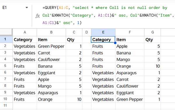
Note: XMATCH searches the header row and returns the correct column number for the given field label.
Sort by Field Name Instead of Column Index in SORT
Using SORT, you typically do this:
=SORT(A2:C, 1, TRUE, 2, TRUE)This sorts by the first and second columns in ascending order, but it’s rigid.
To sort by field label:
=SORT(A2:C, XMATCH("Category", A1:C1), TRUE, XMATCH("Item", A1:C1), TRUE)Cleaner, and much more flexible.
Wrap UP
By using the XMATCH function, you can sort data dynamically based on field labels instead of hard-coded column letters or numbers. This technique is a great step toward more maintainable and readable formulas in Google Sheets.
If you’re working with evolving datasets or collaborating with others, this approach will save you time and avoid formula breakage due to column rearrangement.
Resources
- How to Sort Horizontally (Columns Left to Right) in Google Sheets
- Dynamic Sort Column and Sort Order in Google Sheets
- Sort Names by Last Name in Excel Without Helper Columns
- Sort Column by Length of Text in Google Sheets
- Sort by Custom Order in Google Sheets – How to Guide
- Custom Sort Order in Google Sheets QUERY