


")


")

")
")
 in Excel & Google Sheets")


Smileys and icons can bring life to your spreadsheets if you use them cleverly. You can easily insert smileys and icons based on values in Google Sheets.
Tip: In this guide, “smileys” refer to emoji faces like 😀, 😢, and 😎. Google Sheets lets you use all kinds of emojis — not just faces, but also icons like 🚀, 📈, and 🎯!
For example, you can fill a “Status” column with emojis based on the sales amount of employees:
- If they underperform, show a disappointed face.
- If they meet the target, show a grinning face.
- If they exceed expectations, show a red heart.
You can also use the same method to display other emojis based on values, such as food and drink icons for different menu items or categories.
In this tutorial, I’ll first show you how to insert smileys and icons based on sales values. After that, you’ll naturally be able to apply it to other examples too.
Step 1: Prepare the Example Sheet to Insert Smileys and Icons
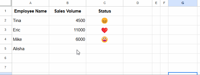
In an empty sheet, let’s prepare the sample data for testing. I have very basic data in Sheet1:
| Employee Name | Sales Volume | Status |
| Tina | 4500 | |
| Eric | 11000 | |
| Mike | 6000 | |
| Alisha | 9500 |
Goal: Display emojis based on sales volume:
- Less than 5000 — 😞 Disappointed face
- Between 5000 and 7499 — 😀 Grinning face
- 7500 and above — ❤️ Red heart
Step 2: Insert Smileys and Icons
You can insert smileys by clicking Insert > Emoji or typing “@” in a cell and selecting Emoji from the shortcut menu.
In Sheet2, column A, insert the smileys and icons you want to use. Here’s how:
- Click Insert > Emoji to open the emoji picker.
- You can browse through different categories like “Smileys & Emotion,” “Animals & Nature,” “Food & Drink,” etc.
- Or, use the search box. For example:
- Search “frowning” to find a sad face.
- Search “rocket” to find a 🚀 rocket icon.
For our example, insert the following in Sheet2:
| Emoji | Sales Threshold |
| 😞 | 0 |
| 😀 | 5000 |
| ❤️ | 7500 |
We are inserting:
- 😞 Disappointed face for underperformance
- 😀 Grinning face for average performance
- ❤️ Red heart for exceeding expectations
Step 3: Assign Conditions to Smileys and Icons Based on Values
Now it’s time to assign sales thresholds to each emoji.
As explained:
- Sales less than 5000 — 😞
- Sales between 5000 and 7499 — 😀
- Sales 7500 or more — ❤️
Enter:
0in B2,5000in B3,7500in B4.
This simple two-column setup is key to inserting smileys and icons based on values in Google Sheets.
Step 4: Insert Smileys and Icons Based on Values Using XLOOKUP
Now let’s dynamically display the emojis based on sales volume!
In Sheet1, cell C2, enter this formula:
=IF(B2="",,XLOOKUP(B2, Sheet2!B:B, Sheet2!A:A, ,-1))Then drag it down.
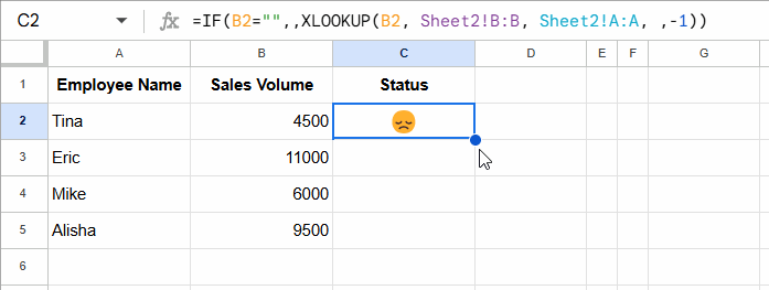
✅ This formula looks up the sales volume from column B, matches it with the correct threshold in Sheet2, and returns the corresponding emoji.
- It finds the largest value less than or equal to the sales amount.
- If there’s no exact match, it finds the next closest smaller number.
Tip: Instead of dragging, you can enter this array formula in C2:
=ArrayFormula(IF(B2:B="",,XLOOKUP(B2:B, Sheet2!B:B, Sheet2!A:A, ,-1)))This automatically fills emojis for all the rows without dragging!
Additional Tip: Inserting Food and Drink Icons Based on Item Names
If you want to show food and drink emojis based on item names, here’s how:
In Sheet2, insert food and drink emojis in column A and corresponding item names in column B.
For example:
| Emoji | Items |
| 🍕 | Pizza |
| 🍩 | Donut |
| 🍣 | Sushi |
| 🍔 | Burger |
Then use this lookup formula in Sheet1:
Single Cell:
=XLOOKUP(B2, Sheet2!B:B, Sheet2!A:A, ,0)Array Formula:
=ArrayFormula(XLOOKUP(B2:B, Sheet2!B:B, Sheet2!A:A, ,0))This matches the item name exactly and returns the corresponding food or drink emoji.
Resources
- Inserting Bullet Points in Google Sheets
- 5-Star Rating in Google Sheets Including Half Stars
- Rate with Ease: Google Sheets’ New Built-In Rating Feature
- Insert Special Characters Without Add-on in Google Sheets
- How to Insert Subscript and Superscript Numbers in Google Sheets
- Conditional Format a Chessboard Pattern in Google Sheets
- 25 Popular Chat Short Words aka Chat Slang That You May Love to Use
- Create a Habit Tracker in Google Sheets: Step-by-Step Guide
Hi, I have tried the formula for the emoji icons to reflect.
However, only the first row reflects the emoji icons and not the following row. Not too sure where the error occurs.
Hi, Deanna,
I could help if you share an example Sheet.
Is there a way to achieve the same result by adding a condition to match the text in the cell?
I’m trying to add an image based on text in the previous cell.
Hi, Paola Soto,
I don’t know what exactly you are trying to achieve.
Try using the image lookup or share a sample sheet.
Thank you very much!
I tried using image lookup. But since I’m starting to learn to work with Google Sheets, I think I wrote it wrong. It keeps saying ERROR.
Here is the sheet: Link removed by admin.
Hi, Paola Soto,
Please see the tabs “kvp test” and “kvp test 2” added to your sample sheet
Hi! so I’ve done this manual conditional formatting to my chart and it looks great!
My only problem is when I try to copy-paste it to a google slide. It does not paste it, even if I don’t link it to the original source. Have you found a solution for this?
Thanks!!