


We can apply the search a value and offset cells concept in a column or row in Google Sheets.
This post explains how to return a value from the left or right of a search value. The result can be from the same row or a different row.
If your requirement is something different, I mean to search in a column; please see if the below two tutorials help.
- How to Filter Next Row to the Filter Criteria Row in Google Sheets.
- How to Offset Match Using Query in Google Sheets.
To search for a value, I won’t use the SEARCH function. Instead, I will use the FILTER function.
Using FILTER, we can easily search a value and offset cells to the left or right of the found value in Google Sheets. Here is how.
See a sample data below just for the example purpose.
I know it’s not coming close to realistic data or resembles. But would be enough to learn the technique.
We may sometimes arrange data like above. I mean month names in one column and corresponding values in the next column.
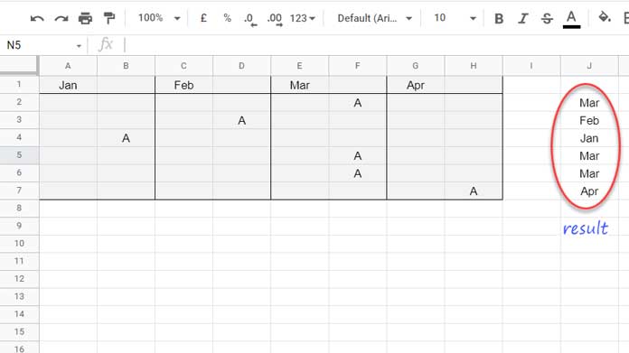
Assume I want to search the value “A” in row # 2 and return its header.
In the usual case, the result would be blank as F1 is blank.
What I want is to offset one cell to the left and return “Mar” from E1.
In the next row, i.e., in row # 3, I want to repeat the same and return the value “Feb” and so on.
I have shown my expected result in J2:J7 (please refer to image # 1 above).
Related: Hlookup to Search Entire Table and Find the Header in Google Sheets – In this tutorial, you will find links to two more similar tutorials.
In the above example, my formula returns the value from the header row after offsetting one cell.
You can choose the same search row instead of the header row to offset and return value.
Let’s see how to search a value and offset cells to their left or right in Google Sheets.
Search a Value and Offset Cells to the Left in Google Sheets
As I have mentioned at the beginning, the simple function here is the FILTER.
We want the offset value from row # 1.
If we don’t want to offset cells to the left or right of the search key, we can use the below formula.
=filter($A$1:$H$1,A2:H2="A")This will return a blank. If you put any value in cell F1, the formula will return that value.
We want to offset one cell to the left. So we can modify the FILTER as below.
=filter({0,$A$1:$H$1},{A2:H2,0}="A")Insert this formula in cell J2 (as per image # 1 above). Then, drag down this formula.
This way, we can search a value in each row and offset cells to the left of the found value in the header row.
If you want to offset two cells to the left, inset one more zero within both the arrays (array 1 is the range and array 2 is the condition) in the formula.
=filter({0,0,$A$1:$L$1},{A2:L2,0,0}="A")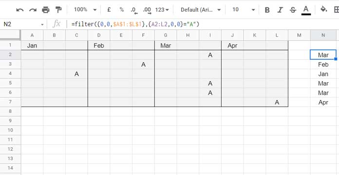
Search a Value and Offset Cells to the Right in Google Sheets
Here there are not many changes. Here we should form the two arrays (range and condition) in the formula differently.
In the above formula, the zeros are prefixed to the result row (range) and suffixed to the search row (condition).
Here it is just the opposite of it. I hope the following formula is self-explanatory.
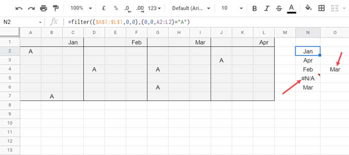
=filter({$A$1:$L$1,0,0},{0,0,A2:L2}="A")This formula searches the value “A” in row # 2 and offsets 2 cells to the right in the first (header) row.
How to Remove the #N/A and Handle Multiple Values
Please see the screenshot above.
The formula returns two values in row # 4 since there are multiple matches in the search.
If you want only the first match, use the INDEX as below.
=index(filter({$A$1:$L$1,0,0},{0,0,A2:L2}="A"),0,1)If you want all the values, use TEXTJOIN.
=textjoin(", ",true,filter({$A$1:$L$1,0,0},{0,0,A2:L2}="A"))What about the #N/A error, then?
Just wrap the formula with IFNA.
Use the above formulas to search a value and offset cells in Google Sheets.
The HLOOKUP Version
We can replace the FILTER formula with an HLOOKUP. But it won’t return multiple offset values.
I prefer FILTER to HLOOKUP as the former is easy to understand and can return multiple offset result values.
If you are curious and want to learn the HLOOKUP use in the above case, here is that example.
Let’s use the HLOOKUP to search the value “A” and offset two cells to the left in Google Sheets.
=hlookup("A",{{A2:L2,0,0};{0,0,$A$1:$L$1}},2,0)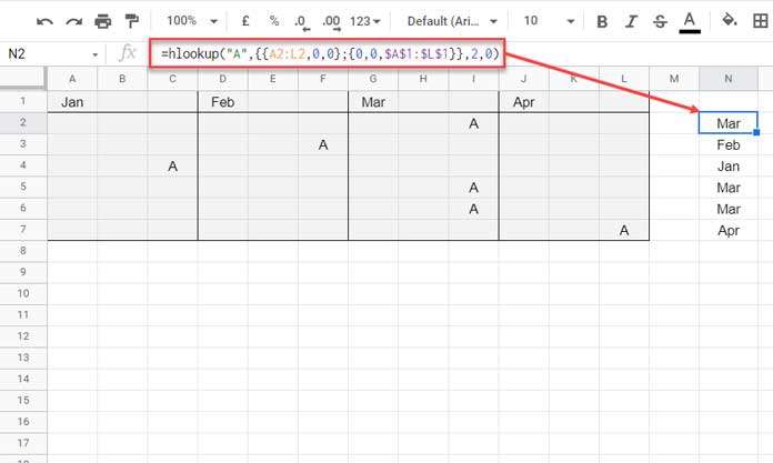
As you can see, the key to offset is modifying the HLOOKUP range by adding extra columns to the right (search row) and left (result row).
In concise, in HLOOKUP;
To search and offset two cells to the left, modify the first row in the range by suffix two extra cells and the second row by prefix two extra cells.
To search and offset two cells to the right, modify the first row in the range by prefix two extra cells and the second row by suffix two extra cells.
That’s all. Enjoy.