I hope this tutorial helps you easily create a scatter chart in Google Sheets. I’ve included all the necessary steps to plot a Scatter Chart in Google Sheets.

You can visualize your data using different types of charts. But if you know which chart type is best suited to your data, creating the chart is just a few clicks away.

In one of my earlier tutorials, I provided insights into chart types and data formatting in Google Sheets, which might be helpful as you make your decision.

Tip: Choose the Suitable Chart for Your Spreadsheet Data – How To

Scatter Chart vs. Line Chart: Which One Should You Use?

When working with your dataset, have you ever wondered, “Should I use a scatter chart or a line chart?” I’ve asked myself this question too!

While both chart types look similar, especially when the dots in a scatter chart are connected using lines, there’s a key difference.

Major Difference Between Scatter Chart and Line Chart

• Line Chart: Best for showing trends over time or comparing trends of multiple series over time.
• Scatter Chart: Best for showing relationships between two variables.

This simple rule can help you decide which chart to use.

A scatter chart has two axes (X and Y), but unlike a line chart, both axes in a scatter chart always represent numerical values. In contrast, the x-axis of a line chart can represent categories or time-based data.

Another name for a scatter chart is an XY graph, which gives you a clear idea of its purpose: visualizing relationships between two variables.

How to Plot a Scatter Chart in Google Sheets

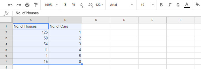
Sample Data:

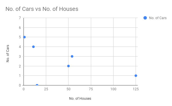
Let’s visualize the relationship between the number of houses in a locality and the number of cars per household in that locality.

Steps to Create a Scatter Chart

1. Select the data range A1:B7.
2. Go to the menu Insert > Chart.
3. In the chart editor panel, under the Setup tab, select Scatter Chart.
4. Ensure the following settings are configured:
   • X-axis: No. of Houses
   • Series: No. of Cars
   • Switch Rows/Columns: Unchecked
   • Use Row 1 as Headers: Checked
   • Use Column A as Labels: Checked
   • Treat Labels as Text: Unchecked
5. Optionally, navigate to the Customize tab to:
   • Add chart and axis titles.
   • Change series colors.
   • Adjust the minimum and maximum values for the horizontal and vertical axes.

By following these steps, you can easily create a scatter chart in Google Sheets to visualize your data effectively.

Similarly, you can plot a scatter chart showing relationships such as the monthly salaries of employees and their monthly rent.

Trendline in Scatter Charts

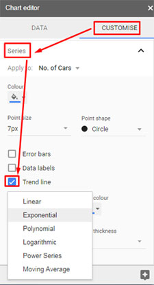
In Google Sheets, you can easily add a trendline to your scatter chart. To do this:

1. Go to the chart editor Customize tab.
2. Click Series.
3. Select the data series and enable the Trendline option. You can choose a linear trendline or other types, depending on your data.

Key Points Recap

• A scatter chart in Google Sheets is perfect for visualizing relationships between variables.
• Unlike line charts, scatter charts always use numerical values for both the x-axis and y-axis.

Additional Resources

• Google Sheets – Add Labels to Data Points in Scatter Chart
• Common Errors You May Encounter in Scatter Chart in Google Sheets
• Conditional Coloring of Data Points in Scatter Charts in Google Sheets