


")


")

")
")
 in Excel & Google Sheets")


When analyzing data in Google Sheets, you may often need a running total by category that resets for each group—for example, tracking sales by product type, expenses by department, or transactions by client. A standard cumulative total adds values continuously across all rows, but in many cases, you’ll want the total to restart whenever the category changes.
In this guide, we’ll cover two formula approaches to calculate a category-wise running total (cumulative total by category) in Google Sheets:
- SUMPRODUCT (and its array version) – works with both sorted and unsorted datasets.
- SUMIF-based formula – works with sorted/grouped datasets and is more efficient for large datasets.
By the end, you’ll know how to create dynamic, accurate running totals for any category in Google Sheets—whether your categories are grouped or scattered.
Sample Data and Expected Output
The sample data is in A1:C, with categories in A2:A and amounts in B2:B. Column C2:C contains the running totals by category, calculated using the formulas we’ll introduce.
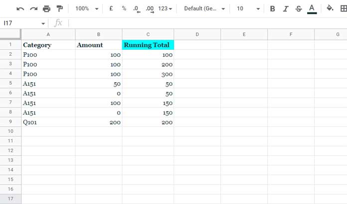
As you can see, the categories are grouped together, but this isn’t required. The formulas below also work correctly when categories are scattered throughout the dataset.
Running Total by Category (Works with Scattered or Grouped Categories)
The simplest method is to use a SUMPRODUCT formula.
=SUMPRODUCT($B$2:$B2, $A$2:$A2=A2)Enter this in cell C2 and drag it down.
How it works:
$A$2:$A2=A2→ checks whether each row’s category (up to the current row) matches the current category.- This returns TRUE (1) or FALSE (0).
- Multiplying that by the amounts and summing the results gives the running total per category.
This formula works reliably with both sorted and unsorted categories, making it versatile for different types of datasets. It’s also straightforward to use, so even beginners can apply it without much effort.
Array Version (No Dragging Required)
If you prefer a formula that automatically spills down, use this:
=MAP(A2:A, B2:B, LAMBDA(cat_, amt_, IF(cat_="",,SUMPRODUCT(B2:amt_, A2:cat_=cat_))))Enter it in C2 after clearing column C.
This is essentially the same drag-down formula, but applied across the full range using MAP. The IF(cat_="",,) ensures blank rows return blank instead of zeros.
⚠️ Drawback: This approach can become resource-intensive and may not perform well with hundreds or thousands of rows. In such cases, the next method is better.
Running Total by Category (Works with Grouped Categories)
If your categories are grouped or sorted, a SUMIF-based formula is faster and scales better for large datasets.
=ArrayFormula(LET(
  uniq, TOCOL(UNIQUE(A2:A), 1),
  seq, SEQUENCE(ROWS(uniq)),
  catg, XLOOKUP(A2:A, uniq, seq),
  IF(A2:A="",,
    SUMIF(ROW(B2:B),"<="&ROW(B2:B), B2:B) - SUMIF(catg,"<"&catg, B2:B)
  )
))
Formula Breakdown
uniq→TOCOL(UNIQUE(A2:A), 1)extracts unique categories, ignoring blanks.seq→SEQUENCE(ROWS(uniq))generates sequence numbers (1, 2, 3, …) for those categories.catg→XLOOKUP(A2:A, uniq, seq)assigns each row’s category a sequence number.
For example:

SUMIF(ROW(B2:B),"<="&ROW(B2:B), B2:B)→ calculates the normal cumulative sum.SUMIF(catg,"<"&catg, B2:B)→ subtracts the cumulative sum of all previous categories (based on their sequence).
The result is a running total that resets for each category.
This formula is the best choice for large, sorted, or grouped datasets, as it runs much more efficiently. It’s also significantly lighter compared to the MAP + SUMPRODUCT array version, making it ideal when performance matters.
Final Thoughts
Creating a running total by category in Google Sheets is simple once you pick the right formula for your dataset size and structure:
- Use SUMPRODUCT drag-down for small to medium datasets with scattered or grouped categories.
- Use the array version (MAP + LAMBDA) if you prefer automation, but only for moderate datasets.
- Use the SUMIF-based array formula for large, sorted/grouped datasets where performance matters.
With these methods, you can calculate cumulative totals by category for products, departments, clients, or any other group—without worrying about dataset size or order. This makes it easier to analyze trends, track progress, and summarize category-wise performance directly inside Google Sheets.