This tutorial explains how to solve the complex task of creating a running sum with the negative value carryover in Google Sheets.

Negative value carryover refers to the process of taking a negative value from one entry and applying it to the next positive value in a sequence.

In the context of a running sum, this means if you encounter a negative value, it is added (as a negative) to the subsequent positive value until the carryover value becomes positive.

Example: The sequence is 5, 50, -5, 10 and the output will be 5, 50, -5, 5.

If there are multiple consecutive negative values, their running sum is calculated and added to the subsequent positive value until the carryover value becomes positive.

Example: The sequence is 5, 50, -5, -10, 4, 20 and the output will be 5, 50, -5, -15, -11, 9.

When a negative value is encountered, it’s essentially treated as a “debt” to be paid off by future positive values. This “debt” is accumulated until a positive value is large enough to cover it.

Creating a running sum with negative value carryover can be useful in several real-life scenarios in Google Sheets, such as:

• Managing inventory levels where stock shortages need to be compensated by subsequent stock additions.
• Adjusting payment schedules where missed payments need to be rolled over and accounted for in subsequent payments.
• Managing utility bills such as electricity, water, etc. where excess usage (negative values) in one period is balanced by savings (positive values) in subsequent periods.

Formula Example of Running Sum with Negative Value Carryover

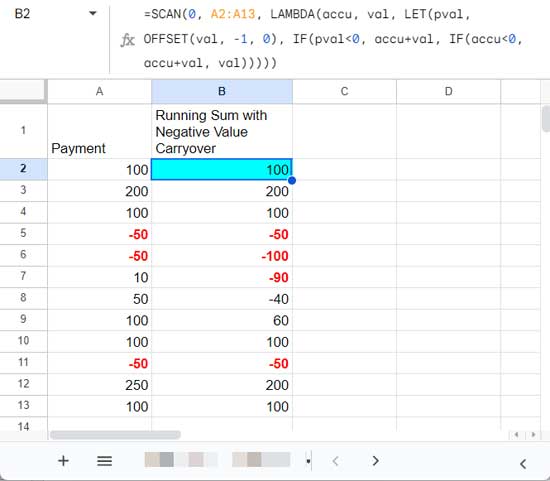
The following sample dataset incorporates a mix of positive and negative values in column A, including consecutive negative values, to effectively showcase the calculation of the adjusted running sum.

You can see the running sum with the negative value carryover in column B, calculated using a formula in Google Sheets.

While the SCAN function provides an elegant and efficient solution for calculating the adjusted running sum with negative value carryover, the complexity of the calculation makes it challenging to replicate using traditional helper column methods. Therefore, we will resort to using SCAN for our purpose.

Steps:

1. Enter the above data (the first column only) in cells A1:A13.
2. Insert the following formula in cell B2:

=SCAN(0, A2:A13, LAMBDA(accu, val, 
   LET(
      pval, OFFSET(val, -1, 0), 
      IF(pval<0, accu+val, IF(accu<0, accu+val, val))
   )
))

The formula breakdown below is optional.

Explanation of the Formula

=SCAN(0, A2:A13, LAMBDA(accu, val, 
   LET(
      pval, OFFSET(val, -1, 0),  // Previous value
      IF(pval<0, accu+val,  // If previous value is negative, add the current value to the accumulator
         IF(accu<0, accu+val,  // If accumulator is negative, add current value to it
            val  // Otherwise, return the current value
         ))
   )
))

Let me explain this formula step by step. Then we will see how to reset the running sum with the negative value carryover based on a category column.

The formula uses the SCAN function to scan the range A2:A13 and produce intermediate results.

The syntax is as follows:

SCAN(initial_value, array_or_range, LAMBDA(name1, name2, formula_expression)

Where:

• initial_value: 0
• array_or_range: A2:A13
• LAMBDA(name1, name2, formula_expression): Please see the explanation below.

You can specify two names in the LAMBDA where name1 represents the accumulator value and name2 represents the current element (value) in the array. So, the assigned names are accu (name1) and val (name2).

The formula expression is:

LET(pval, OFFSET(val, -1, 0), IF(pval<0, accu+val, IF(accu<0, accu+val, val)))

The purpose of the LET function is to name the value expression OFFSET(val, -1, 0) with pval (previous value).

• pval represents the previous value (element) in the array. The OFFSET function offsets -1 row and 0 columns to extract the previous value in the array.

Here is the key part of the formula, a nested IF, that creates a running sum with the negative value carryover:

IF(pval<0, accu+val, IF(accu<0, accu+val, val))

• IF(pval<0, accu+val, …): If the previous value is less than 0, add the accumulator and current value and return it. This returns the running sum of consecutive negative values (leaving the first negative value) and adds the running sum (which is negative) to the next positive value.

IF(accu<0, accu+val, …): If the accumulator value is less than 0, add the accumulator and current value and return it. This adds the negative value carryover (the value in the accumulator) to the next positive value.

Return the current value in all other cases.

Running Sum with Negative Value Carryover and Category Reset

How do we stop the negative value carryover adjustment at the beginning of each category?

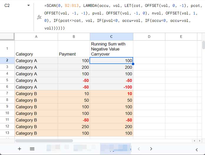
In the following example, we have an additional column called “Category” and the table structure is Category and Payment in columns A and B.

Apply the following formula in cell C2:

=SCAN(0, B2:B13, LAMBDA(accu, val, 
   LET(
      cat, OFFSET(val, 0, -1), pcat, OFFSET(val, -1, -1), 
      pval, OFFSET(val, -1, 0), nval, OFFSET(val, 1, 0), 
      IF(pcat<>cat, val, IF(pval<0, accu+val, IF(accu<0, accu+val, val)))
   )
))

Note: When you use this formula, specify the numeric range B2:B13. The formula will fetch the category by offsetting from this column.

How does this formula differ from our previous non-category formula?

(You can skip this formula explanation part)

To reset the value in each new category row in the accumulator to the current value, you need to find the current and the previous values in the category, then apply the logic IF(previous_row_category <> current_row_category, current_row_value).

This will reset the accumulator in each new category row to the current value.

The additions in this formula are assigning names cat and pcat to the current category and previous row category within the LET function:

cat, OFFSET(val, 0, -1) // current category
pcat, OFFSET(val, -1, -1) // previous category

and the following logical test within the formula expression part:

IF(pcat <> cat, val, ...) // resets the accumulator value to the current value

Error Handling

The running sum with negative value carryover formula usually doesn’t return any errors. Here are some minor points that may help if you run into issues.

I have used closed ranges in the formulas, which are A2:A13 in the first and B2:B13 in the second. If you have a growing range, you can use A2:A or B2:B respectively.

However, if the last value in the accumulator is negative, it can cause issues as the value may be repeated in each blank row below.

Blank cells within the values likely cause no issues since the system considers them as 0s.

The formula uses the SCAN function, which may slow down your sheet’s performance in very large datasets. So, delete all unwanted data from the sheet and remove empty rows and columns.

Resources

We have a collection of resources on running totals in Google Sheets. Check them out below.

• Array Formula for Conditional Running Total in Google Sheets
• How to Calculate a Horizontal Running Total in Google Sheets
• How to Calculate Running Balance in Google Sheets (SUMIF and SCAN Solutions)
• Normal and Array-Based Running Total Formulas in Google Sheets
• Reset Running Total at Blank Rows in Google Sheets
• Reset Running Total at Every Year Change in Google Sheets (SUMIF Based)
• Reverse Running Total in Google Sheets (Array Formula)
• Running Total by Category in Google Sheets (SUMIF Based)
• Running Total with Monthly Reset in Google Sheets (Array Formula)
• Running Total with Multiple Subcategories in Google Sheets
• Weekly and Biweekly Running Totals in Google Sheets