To get rolling 7 days, 30 days, or 60 days data in the Pivot Table, you can use the following workaround in Google Sheets.

In the workaround;

1. We will use a helper cell to input rolling n days.
2. Also, we may use an array formula that will return TRUE or FALSE values in a column in the source of the Pivot Table.

When we input 7, 30, 60, or n days in the helper cell, the Pivot Table data will expand or scale down to that date range.

This method is much faster as you don’t need to open the Pivot Table editor each time to enter a custom formula in the Filter custom formula field.

In addition to the above helper cell and formula, to get rolling 7 days, 30 days, or 60 days in the pivot table in Google Sheets, we can either use the Slicer or Pivot Table Filter itself.

In the below live example, I have used the Pivot Table Filter field, not the Slicer.

How to Get Rolling 7, 30, 60 Days in Pivot Table in Google Sheets

Sample Data

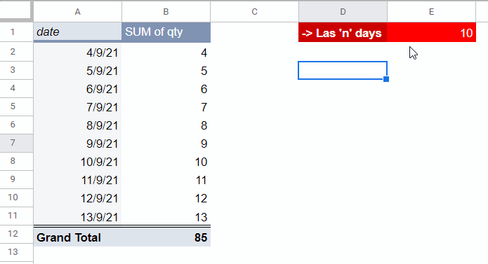
In my workbook (Google Sheets file), I have two sheets named “Source” and “Pivot Table.”

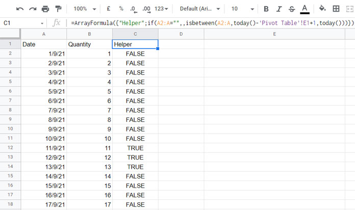
1. Source

It contains the Source Data in the range A1:C.

The actual data range is A1:B. But an array formula in cell C1 populates Boolean values TRUE/FALSE in column C.

So we must consider A1:C as the Pivot source.

Here is the content and the formula in the Source sheet.

=ArrayFormula(
{"Helper";
     if(
        A2:A="",,isbetween(A2:A,today()-'Pivot Table'!E1+1,today())
     )
}
)

Note:- I’ll explain this formula after a few paragraphs below.

2. Pivot Table

This sheet contains the Pivot Table and the helper cell E1 that controls rolling 7, 30, 60, n days in the Pivot Table (please see the above live screenshot).

Formula Explanation

There are two main parts in the formula and they are IF and ISBETWEEN.

IF part:-

Syntax: IF(logical_expression, value_if_true, value_if_false)

The IF part of the formula tests whether A2:A is blank (logical_expression).

If blank (value_if_true), it will return blank else it will execute the ISBETWEEN formula (value_if_false).

ISBETWEEN Part:-

Syntax: ISBETWEEN(value_to_compare, lower_value, upper_value, [lower_value_is_inclusive], [upper_value_is_inclusive])

The arguments within square brackets are optional, and we haven’t used that in our formula.

The ISBETWEEN tests whether the dates in B2:B (value_to_compare) are between today() (upper_value) and today()-‘Pivot Table’!E1+1 (lower_value).

It returns TRUE or FALSE based on the evaluation of the dates in B2:B.

I have already explained ‘Pivot Table’!E1 controls rolling 7, 30, 60 days data in Pivot Table in Google Sheets.

Setup Filter in Pivot Table or Slicer for Getting Rolling 7, 30, 60 Days Data

As I have already mentioned, we can either use the Slicer or Pivot Table filter field.

If you don’t want to use the Slicer, then do as follows.

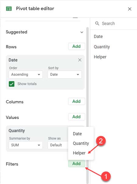
1. Go to the Pivot Table editor.
2. Click on “Add” against “Filter” and select “Helper.” (it’s the column returned by our array formula in the “Source” sheet).
3. It will add the “Filter” field. Click on it and uncheck “FALSE.”
4. Click OK and voila!

The Pivot Table will expand or shrink its size based on the number that you enter in cell ‘Pivot Table’!E1.

This way, you can get rolling 7, 30, 60 days data in Pivot Table without using Slicer in Google Sheets.

If you want to use the Slicer instead of adding Filter within Pivot Table, do as follows.

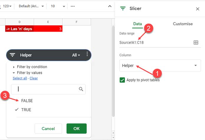
1. Click on the very first cell in the Pivot Table report. As per my example, it’s ‘Pivot Table’!A1.
2. Go to the menu Data > Slicer.
3. Within the Slicer editor panel, select “Helper” as the column. Then set the range as Source!A1:C.
4. Uncheck “FALSE.”
5. Click “OK.”

This way, we can get rolling 7, 30, 60 days data in Pivot Table in Google Sheets.

Thanks for the stay. Enjoy!

Example Sheet 13921

Additional Resources:

• Filter by Date Range Using Filter Menu in Google Sheets.
• Get Last 7, 30, and 60 Days Total in Each Row (from Today) in Google Sheets.
• Filter Data Based on This Week, Last Week, Last 30 Days in Google Sheets.
• Formula to Filter Rolling N Days | Months in Google Sheets.
• Rolling Months Backward Summary in Google Sheets.