


")


")

")
")
 in Excel & Google Sheets")


This tutorial answers how to calculate reverse percentage in Google Sheets.
Below, you’ll find three formulas to calculate the reverse percentage in Google Sheets. Wondering why there are three?
It’s because the formulas vary depending on your requirement, though their purpose is the same: to work backward to find the original number.
Let’s look at an example.
Suppose the price of an item is $100.00. Last month, the vendor was offering a 15% discount on it. Now, instead of a discount, the price has increased by 15%.
So, we have three different prices:
- 15% of the Price = $15.00 (basic). Here, $15.00 is 15% of the original price.
- Discounted Price = $100.00 – $15.00 = $85.00 (price decrease). Here, the final price is $85.00 after a 15% discount.
- Increased Price = $100.00 + $15.00 = $115.00 (price increase). Here, the final price is $115.00 after a 15% hike.
If you have any of these prices — $15.00, $85.00, or $115.00 — you can use a suitable reverse percentage in Google Sheets formula to find the original price.
Here’s a real-life example.
Formulas to Calculate Reverse Percentage in Google Sheets
1. Basic Formula — Inputs are Final Number and Percentage That Made It
Imagine you remember receiving a $195.00 discount when you bought a sofa set for your living room last year, but you forgot the original purchase price.
Since you know the discounted amount (final number) and the percentage it represented of the original price, you can use the following reverse percentage formula in Google Sheets:
Generic Formula:
Final_Number ÷ Percentage = Original Number
In a cell, enter:
=195/15%You’ll get 1300.00, which is the original price of the sofa set.
Want to use cell references instead? Of course!
A1 = 195
B1 = 15%
C1 = =A1/B1
2. Reverse Percentage When You Have Final Number and Percentage Decrease
Sometimes, we apply a discount to a value and later want to find the original value. In that case, here’s the method you need.
Assume you bought a sofa for $1105.00 after a 15% discount. How do you find the original price?
Generic Formula:
Final_Number ÷ (1 – Percentage) = Original Number
In a cell, enter:
=1105/(1-15%)The output will be 1300.00, the original price without the discount.
Prefer to use cell references? Here’s how:
=E2/(1-E3)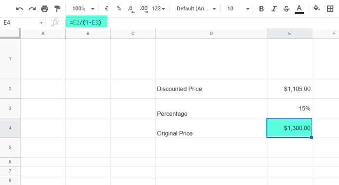
This is a very handy reverse percentage in Google Sheets formula for discount scenarios!
3. Reverse Percentage When You Have Final Number and Percentage Increase
You’ve been dreaming about a car for a long time. Then you read about price hikes coming into effect from the new year — but you didn’t act fast enough!
Now the price has gone up by 3%, and the current price of the model you were eyeing is $29,315.00.
How do you find the car’s price before the hike?
Here’s the reverse percentage in Google Sheets formula you need:
Generic Formula:
Final_Number ÷ (1 + Percentage) = Original Number
In a cell, enter:
=29315/(1+3%)Using cell references:
=E2/(1+E3)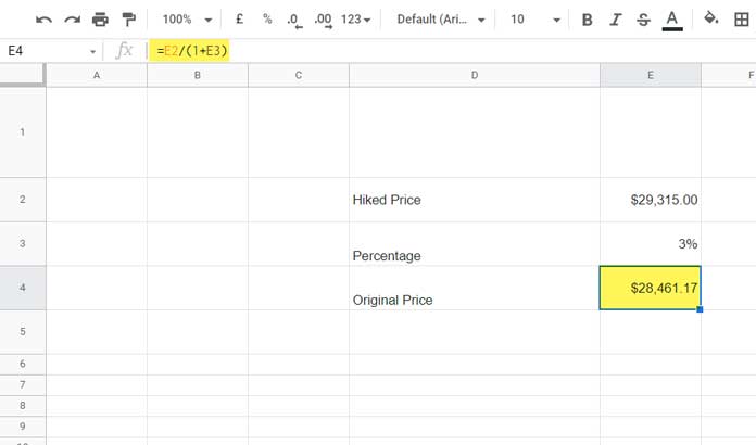
This formula helps you quickly reverse a percentage increase and find the original price.
That’s all. Thanks for staying till the end. Enjoy calculating!
Resources
- How to Use Percentage Value in Logical IF in Google Sheets.
- Percentage Change Array Formula in Google Sheets.
- How to Round Percentage Values in Google Sheets.
- How to Create Percentage Progress Bar in Google Sheets.
- Calculating the Percentage of Total in Google Sheets [How To].
- How to Limit a Percentage Value Between 0 and 100 in Google Sheets.
- Calculating the Percentage between Dates in Google Sheets.
- How to Calculate Percentage Difference In Google Sheets.