


")


")

")
")
 in Excel & Google Sheets")


Replacing blank cells with 0 in a QUERY pivot in Google Sheets can significantly improve data readability and interpretation. You can achieve this easily by leveraging modern Google Sheets functions such as LET or MAP.
An important point to note is that you don’t need to fully understand the underlying QUERY formula to apply this technique. Whether the formula was written by you or someone else, you can still replace blank cells with 0 in the QUERY pivot output without modifying the original QUERY formula. Instead, this approach uses a simple wrapper to substitute blanks with zero values.
Part of the QUERY Pivot & Reporting in Google Sheets series, this tutorial explains how to handle blank or missing values in QUERY pivot results in a clean and non-invasive way.
To demonstrate the concept, we’ll work with a sample dataset containing text, number, and date columns. This will help you see how the formula replaces blank numeric cells with 0 while leaving text and date values unaffected.
Sample Data and QUERY Formula: Setting Up Your Example Sheet
Let’s work with a minimal sample dataset featuring three data types: Date, Text, and Number.
In the provided sample data (please refer to the image below), column A holds the payment made date, column B contains the item or the type of expense, and column C holds their corresponding amounts.
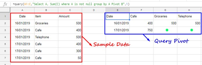
The following QUERY formula in cell E1 generates a Pivot table, organizing payment dates in rows, items in columns, and aggregating the payment amounts.
=QUERY(A1:C, "Select A, Sum(C) where A is not null group by A Pivot B", 1)See the two green dots (manually placed) in the QUERY Pivot output. How do we fill those blank cells with 0? Of course, we can’t enter 0 in those cells because that will break the QUERY formula. Let’s go to our solutions.
You May Like: Learn Google Sheets Query Function: Step-by-Step Guide.
Replacing Blank Cells with 0 in a QUERY Pivot Using the MAP Function
The MAP function is a useful LAMBDA helper function in Google Sheets, allowing us to map each value in an array to a new one.
In this context, the array is the result of a QUERY formula, such as a Pivot table. By employing the MAP function, we can iterate through each value in the Pivot table and replace any blank cells with zero.
Syntax:
MAP(array1, [array2, …], lambda)Generic Formula:
=MAP(array1, lambda(cell_value, IF(cell_value="", 0, cell_value)))Simply substitute array1 with your specific QUERY formula.
For example, in my case, the formula to replace blank cells with 0 values would be:
=MAP(QUERY(A1:C, "Select A, Sum(C) where A is not null group by A Pivot B", 1), lambda(cell_value, IF(cell_value="", 0, cell_value)))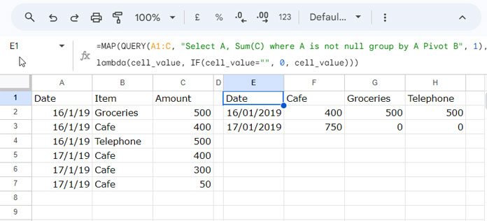
Note: The formula will convert dates to date values. Therefore, select the dates in the Pivot table and apply Format > Number > Date.
This formula effectively transforms the specified QUERY result, replacing any blank cells with 0 while leaving other values unaffected.
Formula Breakdown:
QUERY(A1:C, "Select A, Sum(C) where A is not null group by A Pivot B", 1)
This serves as the array or range of values that you intend to manipulate.lambda
This is a function defining the transformation to be applied to each element in the array.cell_value
It is a user-defined name within the lambda function, representing each cell value in the array.IF(cell_value="", 0, cell_value)
This IF logical test is the lambda function. It takes each cell_value from QUERY Pivot as input and applies the following logic:IF(cell_value="", 0, cell_value)
Replacing Blank Cells with 0 in a QUERY Pivot Using the LET Function
The LET function facilitates the evaluation of formula expressions by using declared named arguments.
Syntax:
LET(name1, value_expression1, [name2, …], [value_expression2, …], formula_expression)Generic Formula:
LET(name1, value_expression1, ArrayFormula(IF(name1="", 0, name1)))In this generic formula, replace value_expression1 with your QUERY formula.
For instance, to replace empty cells with zero in a QUERY Pivot, you can use the following formula:
=LET(name1, QUERY(A1:C, "Select A, Sum(C) where A is not null group by A Pivot B", 1), ArrayFormula(IF(name1="", 0, name1)))Just like the MAP formula, here as well, you need to format the date values to dates in the Pivot result.
Formula Breakdown:
name1: This is the name assigned to the QUERY formula (value_expression1). You can choose a more meaningful name, like “query_formula.”QUERY(A1:C, "SELECT A, SUM(C) WHERE A IS NOT NULL GROUP BY A PIVOT B", 1): The formula (value_expression1) whose result can be referred to later withname1that was declared before.ArrayFormula(IF(name1="", 0, name1)): This expression is evaluated using the LET function. It checks if the value ofname1is an empty string. If true, it returns 0; otherwise, it returns the original value ofname1.
Conclusion
Given that you now have two solutions to replace blanks with 0 in Query Pivot, you might find yourself a little uncertain about which one to opt for.
Feel free to choose either, as both are straightforward formulas and performance-oriented. It’s worth noting that both formulas will convert dates/timestamps to date values. Simply ensure to apply the relevant formatting from the Format menu by selecting those date values.
Related:
I think there is a simpler solution than using a query within the query: use the TEXT function with a “multi” format string.
=ARRAYFORMULA(TEXT(QUERY(...), "0;0;0;@"))Hi, Rehan Ahmad,
Thanks for the formula tip!
Rehan – to enable my pivot table to show “0” instead of blank cells, where would I add your formula to my current formula? I can’t figure it out 🙁
=QUERY('Order Engagment NATIONAL Chart SORTED Data V1'!U5:W,"SELECT V, SUM(W) Where U is Not Null GROUP BY V PIVOT U")Hi, Weston B,
If you follow his suggestion, you can replace your formula as below.
=ARRAYFORMULA(TEXT(QUERY('Order Engagment NATIONAL Chart SORTED Data V1'!U5:W,"SELECT V, SUM(W) Where U is Not Null GROUP BY V PIVOT U"), "0;0;0;@"))The issue is it will convert all the number values to text format.
Here is my suggested formula as per the tutorial.
={query('Order Engagment NATIONAL Chart SORTED Data V1'!U5:W,"SELECT V, SUM(W) Where U is Not Null GROUP BY V PIVOT U limit 0",1)
;
query(query('Order Engagment NATIONAL Chart SORTED Data V1'!U5:W,"SELECT V, SUM(W) Where U is Not Null GROUP BY V PIVOT U",1),"Select Col1 offset 1",0)
,
ArrayFormula(N(query(query('Order Engagment NATIONAL Chart SORTED Data V1'!U5:W,"Select V, Sum(W) where U is not null group by V Pivot U",1),"Select "&textjoin(", ",true,"Col"&sequence(1,countunique(U6:U),2))&" offset 1",0)))
}
Here is my new suggestion:
Syntax:
If(query=space, zero, query).Formula:
=ArrayFormula(if(QUERY('Order Engagment NATIONAL Chart SORTED Data V1'!U5:W,"SELECT V, SUM(W) Where U is Not Null GROUP BY V PIVOT U")="",0,
QUERY('Order Engagment NATIONAL Chart SORTED Data V1'!U5:W,"SELECT V, SUM(W) Where U is Not Null GROUP BY V PIVOT U")
))
Hi Prashanth,
Thanks for all the info on your site, it has been extremely helpful.
I am stuck on one part of a query pivot if you have any ideas to help.
I currently have a formula;
={query(Filter!A:N, "Select G, Count(J) group by G Pivot H limit 0",1); query(query(Filter!A:N, "select G, Count(J) where G is not null group by G Pivot H", 1),"select Col1 offset 1",0), ArrayFormula((N(Query(query(Filter!A:N, "select Count(J) group by G Pivot H",1),"Select * offset 1",0))))}This displays how I want it to and the blanks are now zeros, fantastic.
One further step that I would like to do is to filter by the year, Column J is a year step with the following years 2017, 2018 and 2019.
I would like a different pivot for each year.
Column G is a string with the day of the week, example “1 Sunday” or “4 Wednesday”
Column H is the week number found using Weeknum()
Any help would be much appreciated.
Kind Regards,
Dan
Hi, Dan,
I may require a sample Sheet to test your formula and possibly implement any additional requirement.
Best,
Great, how about when the values are countA? My chart won’t produce because the “column should be numeric” but dumb google sheets returns
""tocountA()instead of zero.Hi,
The Query function doesn’t support the COUNTA aggregation function. If you want me to look into the problem, feel free to share an example Sheet.