")
")


")


")

")
")
 in Excel & Google Sheets")


This tutorial explains how to track the remaining days for your tasks using a Sparkline Gantt Chart in Google Sheets.
The bar will have two colors distinguishing elapsed days and remaining days. The colors are customizable.
Some of the features include:
- Based on the SPARKLINE Function
We’ll use the SPARKLINE function to create the bar chart. Even if you have multiple tasks, you won’t need to write separate formulas for each one. We can simply spill the formula down to automatically populate the Sparkline charts. - Control the Timeline Period
The timeline is flexible. You can specify a project start date, and the chart will automatically populate for a default period, such as 4 weeks, starting from that date. You can then adjust the week number to control from which week after the start date the timeline should begin.
Let’s proceed with the step-by-step instructions to help you track the remaining days of your tasks with a Sparkline Gantt Chart in Google Sheets.
Step 1: Setting Up Your Data and Timeline
This section doesn’t involve any formulas. They will be introduced from the second step onwards, specifically for populating the timescale, calculating duration, elapsed days, and remaining days, and creating Sparklines for tracking remaining days.
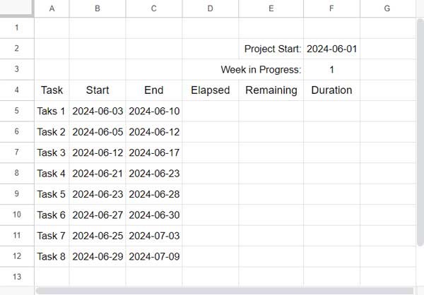
- Enter the task names, start dates, and end dates in columns A4:C, where A4, B4, and C4 contain the corresponding headers “Task,” “Start,” and “End,” respectively.
- In cell F2, enter the project start date. It can be any date, but usually the earliest date in the B column (B5:B), which is the start date column.
- In cell F3, enter the week number, like 1, 2, or 3. This number represents the week number from the start date in cell F2. Based on this number, the timescale formula will populate the dates. We will cover that later.
Step 2: Creating a Dynamic Gantt Chart Timeline
Enter the following formula in cell G3:
=SEQUENCE(1, 28, F2-WEEKDAY(F2,3)+(F3-1)*7)This will populate the timescale, considering the project start date in cell F2, the week number in cell F3, and Monday as the start of the week.
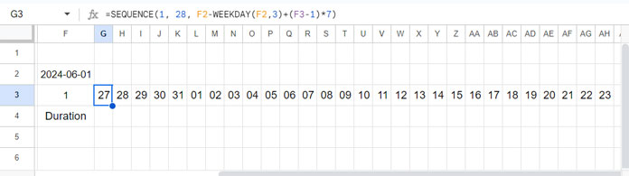
Let’s break down this formula:
Syntax:
SEQUENCE(rows, [columns], [start], [step])In our formula, ‘rows’ is 1, and ‘columns’ is 28, which means a timescale for 28 days (4 weeks). The ‘start’ argument is the key, and here is the breakdown.
F2-WEEKDAY(F2, 3) + (F3 - 1) * 7returns the timescale start, where:F2-WEEKDAY(F2, 3)returns the week start of the project start date. The formula deducts the weekday number of the start date from the start date, where the weekday number for Monday is 0. This ensures the timescale always starts on Monday.(F3 - 1) * 7returns the multiplication of (F3 – 1) by 7, meaning if the week number is 1, the output will be 0; if the week number is 2, the output will be 7, and so on.
The SEQUENCE function returns the numbers 1 to 28 across the row, with the starting value being the calculated start date.
Step 3: Choosing Sparkline Data for Remaining Days
We need three data points to create the Gantt chart with the SPARKLINE function to help you monitor the remaining days.
Offset (Data Point #1):
Let’s understand the ‘offset’ data point.
If the timescale start date in cell G3 is 2024-05-27 and the task start date in cell B5 is 2024-06-03, the ‘offset’ would be 7. If the task start date is before the timescale start date, then there will be no ‘offset’.
=MAX(0, B5-G3)We will use this directly within the SPARKLINE formula.
Duration (Not a Data Point):
Enter the following formula in cell F5 and drag the fill handle down as far as you want.
=LET(start, DATEVALUE(B5), end, DATEVALUE(C5), timeline_start, $G$3, IFERROR(MAX(0, DAYS(end, MAX(timeline_start, start))+1)))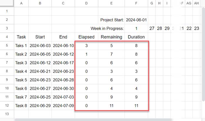
This method calculates the duration by considering the later date between the task’s start date and the timescale start date.
While this ensures the Sparkline bar starts at the correct position on the timeline, it might not always reflect the actual duration of the task based solely on its original start and end dates.
Remaining Days (Data Point #2):
Enter this formula in cell E5 and drag the fill handle down as far as you want.
=LET(start, DATEVALUE(B5), end, DATEVALUE(C5), timeline_start, $G$3, IFERROR(MAX(0, DAYS(end, MAX(TODAY(), MAX(timeline_start, start)))+1)))Similar to duration, the formula for remaining days doesn’t directly use today’s date and the task end date. Here’s how it works:
- Finding the Later Start Date
The formula first identifies the later date between the task’s start date and the timescale start date. - Comparison with Today
It then compares this later start date with today’s date and returns the larger of the two. - Remaining Days Calculation
Finally, the formula subtracts this larger date (either the later start date or today’s date) from the task’s end date to determine the remaining days.
Elapsed Days (Data Point #3):
Enter the following formula in cell D5 and drag the fill handle down as far as you want.
=F5-E5Step 4: Tracking Remaining Days with the Sparkline Formula
To create Sparkline bars for all tasks, we need to merge rows. Here’s how you can do it:
- Select the cells from G5 to AH5.
- Click on “Format” > “Merge Cells” > “Merge Horizontally”.
- Then, select the merged range, right-click, and choose “Copy” from the context menu.
- Next, select cells from G6 to AH12, right-click, and select “Paste”.
In cell G5, enter the following formula to generate Sparkline bars for all tasks:
=MAP(B5:B12, D5:D12, E5:E12, LAMBDA(x, y, z, SPARKLINE({MAX(0, x-G3), y, z},{"charttype","bar";"color1","white";"color2","#A9A9A9"; "color3","#90EE90"; "max", COUNT(G3:AH3)})))This formula uses a custom Lambda function within the MAP function to follow the SPARKLINE syntax: SPARKLINE(data, [options]).
Where:
data:{MAX(0, x-G3), y, z}MAX(0, x-G3): This calculates the ‘offset’ days where ‘x’ represents the task start date (from range B5:B12) – data point #1.y: This represents the elapsed days of each task (from range D5:D12) – data point #2.z: This represents the remaining days of each task (from range E5:E12) – data point #3.
options:{"charttype","bar";"color1","white";"color2","#A9A9A9"; "color3","#90EE90"; "max", COUNT(G3:AH3)}– It defines various aspects of the Sparkline chart.
The MAP function iterates through three ranges of data (B5:B12, D5:D12, and E5:E12) containing task start dates, elapsed days, and remaining days, respectively.
For each set of corresponding values, the MAP function applies the provided Lambda function to generate the Sparkline data and options for that specific task.
This allows the formula to create Sparklines for all tasks in a single formula, rather than needing to write separate formulas for each row.
With this Sparkline Gantt chart, we can easily track the remaining days for each task in Google Sheets.
The current formula uses subtle shades of gray and green to visually represent elapsed days and remaining days, respectively. You can customize these colors within the formula itself.
Resources
- Task Duration, Remaining, and Elapsed Days Calculation: Google Sheets
- Days Remaining in Gantt Chart in Google Sheets
- Create a Gantt Chart Using Sparkline in Google Sheets
- Sparkline Bar Chart Formula Options in Google Sheets
- Sparkline Column Chart Options in Google Sheets
- Sparkline Line Chart Formula Options in Google Sheets
- SPARKLINE for Positive and Negative Bar Graph in Google Sheets
- Elapsed Days and Time Between Two Dates in Google Sheets