Relative reference in conditional formatting is not a matter of concern in Google Sheets if the cell range to highlight and the conditions are within the same sheet. It’s a concern only when they are in two different sheets in the same file!

Unlike normal worksheet formulas, the formulas in conditional formatting, known as formula rules, require the INDIRECT function to refer to another sheet.

As you may know, the INDIRECT function uses a cell reference as a string. So when we use INDIRECT to refer to a cell in Google Sheets in a ‘normal’ way, relative cell reference has no effect.

Syntax: INDIRECT(cell_reference_as_string, [is_A1_notation])

But we can overcome that by using the ROW and COLUMN functions within the ADDRESS function as the cell_reference_as_string argument inside INDIRECT.

In this post, let’s learn how to apply Relative Cell Reference in Conditional Formatting when two sheets are involved in the same Google Sheets file.

Before that, you must know how to apply Relative Cell Reference in Conditional Formatting within the same sheet in Google Sheets.

Relative Cell Reference in Conditional Formatting in the Same Sheet

Relative cell reference helps us use a single conditional format formula across an entire row or column range. So, no need to create separate formula rules for each cell or row/column.

Let me start with a column range, as it’s the most common scenario in conditional formatting.

Formula for a Column Range

Here’s an example. I want to highlight values in A2:A if B2:B is “Pending.” Both values are in the same sheet. How do I do that?

Here is the formula you must insert via Format > Conditional formatting > Format rules, and then select “Custom formula is.”

Custom Formula #1:

=B2="Pending"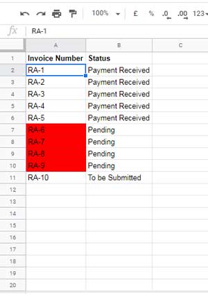

The only thing you need to take care of is the “Apply to range” field inside the “Conditional format rule” panel.

You must set it to A2:A so that the formula for the first cell will automatically apply to the selected range. Because we have used a relative cell reference (no dollar sign with B2).

Suppose I want to highlight both columns A and B. Simply changing “Apply to range” to A2:B won’t yield the desired result.

In such a scenario, make the column (letter) absolute and keep the row (number) relative.

Custom Formula #2:

=$B2="Pending"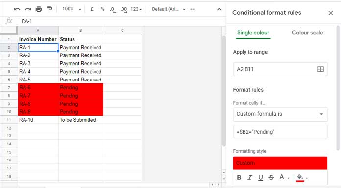

What about if the values are in two rows instead of two columns?

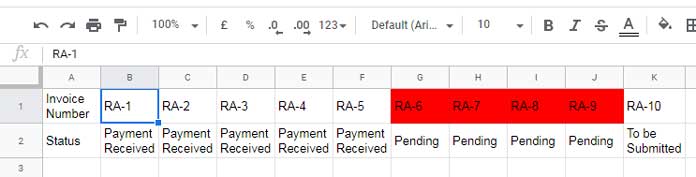
Formula for a Row Range

Here too, there is no change in how we use Relative Cell Reference in Conditional Formatting in Google Sheets.

If the invoice numbers are in row #1 and the statuses are in row #2, the same formula rule #1 applies to highlight row #1.

Just set “Apply to range” to B1:K1 to get the highlighting, as shown below.

To highlight both rows, using custom formula #2 won’t work because the column was made absolute.

Here, instead, we must make the row (number) absolute. Also, change the highlight range to A1:K2.

Custom Formula #3:

=B$2="Pending"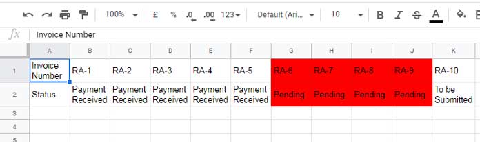

Relative Cell Reference in Conditional Formatting Across Two Sheets

The above custom formulas won’t work if the invoice numbers are in one sheet and the statuses are in another sheet. No matter whether it’s column-wise or row-wise.

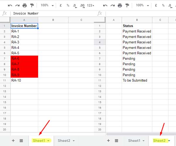
For example, the invoice numbers are in A1:A in “Sheet1,” and the statuses are in B1:B in “Sheet2” (this setup is just for explaining Relative Cell Reference in Conditional Formatting).

In this case, some of you might think the following rule would work:

=Sheet2!B2="Pending"

But it won’t, because conditional formatting rules in Google Sheets only apply within the same sheet. That’s why the workaround is to use INDIRECT.

Whenever two or more sheets are involved in conditional formatting, we must use the INDIRECT function.

(Must Read: Using INDIRECT in Conditional Formatting in Google Sheets.)

Since our focus here is Relative Cell Reference in Conditional Formatting, let me show you how to use INDIRECT properly.

Indirect Formula for a Column Range

In the image below, you can see the values (invoice numbers) to highlight are in “Sheet1,” while the criteria are in “Sheet2.”

Here is the formula to use:

Custom Formula #4:

=INDIRECT("'Sheet2'!"&ADDRESS(ROW(B2),COLUMN(B2),4))="Pending"

To apply relative cell reference highlighting to an entire row (e.g., columns A and B in “Sheet1”), change B2 to $B2 in both the ROW and COLUMN functions inside ADDRESS.

Custom Formula #5:

=INDIRECT("'Sheet2'!"&ADDRESS(ROW($B2),COLUMN($B2),3))="Pending"

Don’t forget to change the “Apply to range” to A2:B.

Indirect Formula for a Row Range

Now let’s assume the values to highlight are in A1:K1 in “Sheet1,” and the conditions are in A2:K2 in “Sheet2.”

If so, use the same Custom Formula #4 above. Just set “Apply to range” to B1:K1.

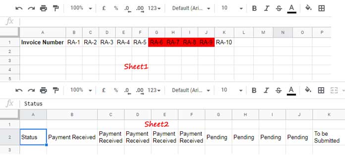
To highlight multiple rows in “Sheet1,” for example, A1:K2, based on the same conditions in “Sheet2,” use this formula:

Custom Formula #6:

=INDIRECT("'Sheet2'!"&ADDRESS(ROW(B$2),COLUMN(B$2),4))="Pending"

That’s all about Relative Cell Reference in Conditional Formatting in Google Sheets.

Thanks for staying till the end. Enjoy!

Additional Resources

• Google Sheets: Dollar Symbols and Relative/Absolute References
• Relative Cell Reference in Importrange in Google Sheets
• Relative Reference in Drop-Down Menu in Google Sheets
• Highlight Values in Sheet2 that Match Values in Sheet1 Conditionally
• Highlight Cells if Same Cells in Another Sheet Have Values
• How to Conditional Format Duplicates Across Sheet Tabs in Google Sheets