In the rank without ties approach, we will assign the superior rank to the first value in a tie. Let’s see how it works in Google Sheets.

There are two rank functions in Google Sheets to assign ranks to numbers in a list: RANK.EQ and RANK.AVG.

At present, none of them have the tie-breaking capability.

When using these functions, if two people have the same score or mark, their rank will be the same.

If there is a tie in ranking because of the same score, mark, etc., the first function will return the same rank, whereas the second function will return the average rank.

That doesn’t mean rank without ties is not possible in Google Sheets. We can use RANK.EQ with COUNTIF for the same.

The above combination will also work with an array formula that spills down from the inserted cell to return rank without ties in a list or array.

First, I am starting with the non-array (drag-down) formula so that you can understand the logic.

Rank without Ties (Non-array Formula)

We can assign rank from top to bottom (descending order) or bottom to top (ascending order).

In descending order, the greatest value in data will have rank 1.

E.g.:- A student who scored 100 out of 100 will be ranked 1, and 99 out of 100 will be ranked 2.

In ascending order, the least value in data will have rank 1.

E.g.:- A student who scored 99 out of 100 will be ranked 1, and 100 out of 100 will be ranked 2.

We usually follow the top to bottom (descending order) approach.

We will start from that in our rank without ties formula example in Google Sheets.

Top to Bottom (Desc. Order)

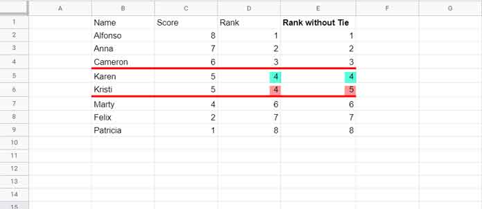
In the above example, the players “Karen” and “Kristi” have the same score, i.e., 5. So the rank of those persons is 4.

Cell D2 has the following formula, which I have copied down until cell D9.

=RANK.EQ(C2,$C$2:$C$9,0)

In the formula, the cell reference C2 is the value, and the cell range $C$2:$C$9 is the data as per the syntax of the function RANK.

RANK.EQ(value, data, [is_ascending])

The value must be in relative reference, whereas the data must be in absolute reference.

Because when we drag down the formula, we want the value reference to change, not the data range reference.

To assign rank without ties in Google Sheets, I have used the below RANK.EQ + COUNTIF combination in cell E2, which copied down.

=RANK.EQ(C2,$C$2:$C$9,0)+COUNTIF($C$2:C2,C2)-1

Please scroll up and see the image.

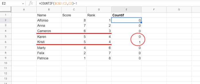
Let’s see what the above COUNTIF does.

The COUNTIF above returns 0 for the first occurrence of a score, 1 for the second occurrence, and so on.

We added these occurrence numbers to the RANK.EQ results to break ties.

Bottom to Top (Asc. Order)

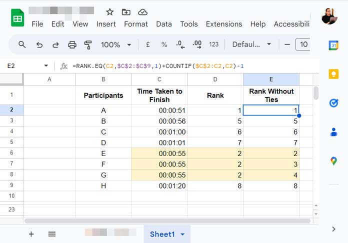
When we want to find the rank of participants in sporting events such as running, horse riding, and auto racing, we should consider ranking based on finishing time (who finished first).

So, the least value (time) in data will rank 1.

Usually, there won’t be a tie in such tight competitions. If there is any, we can use the below formula to rank without ties in Google Sheets.

D2:

=rank(C2,$C$2:$C$9,1)

E2:

=RANK.EQ(C2,$C$2:$C$9,1)+COUNTIF($C$2:C2,C2)-1

I’ve copied both formulas down.

Just specified 1 instead of 0 in the is_ascending part of the RANK.EQ formula. That’s the only change compared to our earlier two formulas.

Array Formula to Rank without Ties in Google Sheets

In the Array Formula, we won’t use COUNTIF. Then?

We will use COUNTIFS. But the logic will be similar to the above non-array formula, i.e., adding occurrences with ranks.

Insert the below formula in cell E2 (please refer to image – 1 above).

=ArrayFormula(
     IFNA(
        rank.eq(C2:C9,C2:C9,0)+
        COUNTIFS(C2:C9,C2:C9,ROW(C2:C9),"<="&ROW(C2:C9))
        -1
     )
)

It will expand the results in the range E3:E9. If the range is not blank, then it will return a #REF error.

Remember! When using this formula, it assigns rank 1 to the greatest value in the data.

Use the below formula if you want the lowest time (value) to get a higher rank (please refer to image # 3).

=ArrayFormula(
     IFNA(
        rank.eq(C2:C9,C2:C9,1)+
        COUNTIFS(C2:C9,C2:C9,ROW(C2:C9),"<="&ROW(C2:C9))
        -1
     )
)

Formula Explanation

In the non-array formula, we have used RANK.EQ and COUNTIF in non-array form. Here, on the contrary, we are using array formulas.

You can find the rank without ties array formula explanation below.

There are two parts to the formula.

Part # 1:

rank.eq(C2:C9,C2:C9,0)

or

rank.eq(C2:C9,C2:C9,1)

Part # 2:

COUNTIFS(C2:C9,C2:C9,ROW(C2:C9),"<="&ROW(C2:C9))-1

Both the above parts use the ArrayFormula function to expand.

The first one returns the rank of all the scores (please refer to D2:D9 in image – 2), whereas the second function returns the count of occurrences (please refer to E2:E9 in the image – 2).

That means Part # 1 is the array formula version of the RANK.EQ. But Part # 2 may be new to you. I have included the Part # 2 details in a separate post here – Running Count in Google Sheets.

As a side note, I have another array solution for the tie-breaking in ranking.

Though the RANK.EQ + COUNTIFS is the simplest one I am sharing that too here – Flexible Array Formula to Rank Without Duplicates in Google Sheets.

That’s all about rank without ties in Google Sheets.

Thanks for the stay. Enjoy!