This tutorial explains how to use OR logical conditions in the same column or across two different columns using the SUMPRODUCT formula in Google Sheets. This will help you master conditional SUMPRODUCT.

The primary purpose of SUMPRODUCT is to find the product of two or more arrays of equal size. However, you can go beyond this core purpose and use it for conditional counting or conditional summation as well. It’s not overly complex if you understand the logic behind it.

SUMPRODUCT with OR Condition in a Single Column

We will use the following material purchase data in the range A1:E to learn how to use OR conditions in the SUMPRODUCT function:

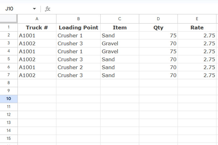
You can use the following formula to count the number of purchases from Crusher 1:

=SUMPRODUCT(B2:B="Crusher 1")

To find the total cost of purchases from Crusher 1, use the formula:

=SUMPRODUCT(B2:B="Crusher 1", D2:D, E2:E)

This calculates the total cost by multiplying the quantities in column D with the rates in column E, only when the Loading Point is Crusher 1.

To count the number of purchases from either Crusher 1 or Crusher 2, use the OR condition in SUMPRODUCT as follows:

=SUMPRODUCT((B2:B="Crusher 1")+(B2:B="Crusher 2"))

To calculate the total purchase cost for both Crusher 1 and Crusher 2, include the Qty and Rate columns:

=SUMPRODUCT((B2:B="Crusher 1")+(B2:B="Crusher 2"), D2:D, E2:E)

That’s how you can use an OR condition in SUMPRODUCT within a single column.

SUMPRODUCT with OR Condition in Multiple Columns

In rare cases, you might need to use the OR condition in SUMPRODUCT across two different columns. Let’s consider the following data in A1:B:

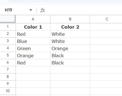
Suppose you want to count rows where Color 1 is “Red” or Color 2 is “White.” You can use the following formula:

=SUMPRODUCT(SIGN((A2:A="Red")+(B2:B="White")))

Explanation of the Formula

• (A2:A="Red"): Returns TRUE for rows where Color 1 is “Red”; otherwise, it returns FALSE.
• (B2:B="White"): Returns TRUE for rows where Color 2 is “White”; otherwise, it returns FALSE.

When you add these two conditions, the possible outcomes are:

• 0: Neither condition is met.
• 1: One condition is met (either “Red” in Color 1 OR “White” in Color 2).
• 2: Both conditions are met (both “Red” in Color 1 AND “White” in Color 2).

The SIGN function ensures that any result greater than 0 (either 1 or 2) is converted to 1, allowing you to count rows where at least one condition is true.

The formula returns 3 in the example above because three rows meet at least one of the conditions.

Final Notes

Using SUMPRODUCT with OR conditions across multiple columns is not a common requirement. However, knowing this technique equips you with the flexibility to handle diverse data scenarios.

Resources

• How to Use Date Differences as Criteria in SUMPRODUCT in Google Sheets
• Differences Between SUMIFS and SUMPRODUCT Functions in Google Sheets
• Comparing SUMIFS, SUMPRODUCT, and DSUM with Examples in Google Sheets
• Correctly Specifying Criteria in SUMPRODUCT in Google Sheets
• How to Do a Case Sensitive SUMPRODUCT in Google Sheets
• How to Use Wildcards in SUMPRODUCT in Google Sheets
• How to Use SUMPRODUCT with Merged Cells in Google Sheets
• SUMPRODUCT Differences: Excel vs. Google Sheets