


")


")

")
")
 in Excel & Google Sheets")


Tracking recurring dates such as anniversaries, subscription renewals, or contract milestones is a common need in spreadsheets. This tutorial will show you how to calculate the next biannual, annual, biennial, and triennial dates in Google Sheets using simple, dynamic formulas.
Why Find Next Recurring Dates in Google Sheets?
You might want to find upcoming event dates to:
- Track your next wedding anniversary
- Calculate the end of a hire purchase agreement
- Schedule a subscription plan renewal
- Plan employee reviews or certification renewals
- Manage equipment maintenance schedules
By entering your start date(s) in a column, you can automatically get the upcoming anniversary or event dates for each entry.
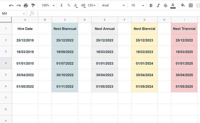
Example
| Today’s Date | Date to Evaluate | Next Biannual | Next Annual | Next Biennial | Next Triennial |
| 30/04/2022 | 18/03/2019 | 18/09/2022 | 18/03/2023 | 18/03/2023 | 18/03/2025 |
Next Biannual, Annual, Biennial, and Triennial Date Formulas
Assuming your dates to evaluate are in the range A2:A, the formulas below calculate the next upcoming dates based on today’s date.
Next Biannual Date Formula in Google Sheets
The Next Biannual Date formula calculates the next recurring date every 6 months from a given start date.
Formula
=ARRAYFORMULA(LET(
  hiredate, A2:A,
  months, IFERROR((YEAR(TODAY()) - YEAR(DATEVALUE(hiredate))) * 12, " "),
  biannual, EDATE(hiredate, months),
  IFERROR(
    IF(
      months <= 0, EDATE(hiredate, 6),
      IF(biannual < TODAY(), EDATE(hiredate, months + 6), biannual)
    )
  )
))
Explanation
hiredateholds the dates you want to evaluate.monthscalculates the total months elapsed since thehiredateyear to this year.EDATE(hiredate, months)calculates the date after adding that many months.- The formula checks if this date is in the past; if so, it adds another 6 months to get the next biannual date.
- It handles cases where the hire date is in the future or today.
Next Annual Date Formula in Google Sheets
The Next Annual Date formula calculates the upcoming yearly recurrence from a start date. It’s perfect for tracking anniversaries, contract renewals, or birthdays.
Formula
=ARRAYFORMULA(LET(
  hiredate, A2:A,
  months, IFERROR((YEAR(TODAY()) - YEAR(DATEVALUE(hiredate))) * 12, " "),
  annual, EDATE(hiredate, months),
  IFERROR(
    IF(
      months <= 0, EDATE(hiredate, 12),
      IF(annual < TODAY(), EDATE(hiredate, months + 12), annual)
    )
  )
))
Explanation
This formula is similar to the biannual one but adds 12 months instead of 6.
- It calculates how many months have passed.
- Returns the next date that falls 1 year or a multiple of years after the hire date.
- Ensures the result is after today.
Next Biennial Date Formula in Google Sheets
Use this formula to find the next date recurring every 2 years (24 months).
Formula
=ARRAYFORMULA(LET(
  hiredate, A2:A,
  months, IFERROR(ROUNDUP((YEAR(TODAY()) - YEAR(DATEVALUE(hiredate))) / 2) * 24, " "),
  biennial, EDATE(hiredate, months),
  IFERROR(
    IF(
      F2:F <= 0, EDATE(hiredate, 24),
      IF(biennial < TODAY(), EDATE(hiredate, months + 24), biennial)
    )
  )
))
Explanation
- Here, months are calculated as multiples of 24 (2 years).
ROUNDUPensures that partial intervals are rounded up to the next biennial period.- This formula tracks events like certifications or contract reviews every two years.
Next Triennial Date Formula in Google Sheets
This formula calculates the next date recurring every 3 years (36 months).
Formula
=ARRAYFORMULA(LET(
  hiredate, A2:A,
  months, IFERROR(ROUNDUP((YEAR(TODAY()) - YEAR(DATEVALUE(hiredate))) / 3) * 36, " "),
  triennial, EDATE(hiredate, months),
  IFERROR(
    IF(
      months <= 0, EDATE(hiredate, 36),
      IF(triennial < TODAY(), EDATE(hiredate, months + 36), triennial)
    )
  )
))
Explanation
- Similar to the biennial formula but using 36 months (3 years).
- Useful for long-term planning, audits, or equipment replacement cycles.
How These Formulas Relate
All these formulas follow a similar structure:
- Calculate how many intervals (months) have passed since the original date.
- Use
EDATEto jump ahead by the corresponding months. - Check if the resulting date is before today; if so, add one more interval.
- Return the next upcoming date for the cycle.
They differ only in the interval length:
| Frequency | Months Interval |
| Biannual | 6 |
| Annual | 12 |
| Biennial | 24 |
| Triennial | 36 |
Summary
Using these formulas, you can dynamically calculate next recurring dates in Google Sheets based on any start date list. This helps automate reminders, scheduling, and planning.
Related Resources
- Get the Next Renewal Date Based on Custom Month Intervals in Google Sheets
- How to Generate Next Available Date in Google Sheets
- Countdown Timers in Google Sheets (Easy Way!)
- Finding the Closest Date to Today in Google Sheets
- Create a Dynamic Date That Advances or Resets in Google Sheets
- Current Quarter and Previous Quarter Calculation in Google Sheets
- Convert Dates to Fiscal Quarters in Google Sheets
- Array Formula to Generate Bimonthly Dates in Google Sheets
Thanks, Prashanth, the formula worked wonderfully. I have a few questions in trying to comprehend the formula. If it is an array formula, should B5 be B5:B, D5 be D5:D, and C5 be C5:C? Why is D5/freq1 necessary in this case? What does the sequence do? Thanks again for your advice.
Q1: “If it is an array formula, should B5 be B5:B, D5 be D5:D, and C5 be C5:C?”
Answer: No, the same cell references can be used. However, to turn it into an array formula, you might need to use the MAP function.
Q2: “Why is D5/freq1 necessary in this case?”
Answer: This is necessary because it facilitates the initial offset by a year (you can also specify 2 years or 3 years, as needed). It controls that part. The freq2 parameter manages the month part.
Q3: “What does the sequence do?”
The SEQUENCE function generates a sequence of dates based on “freq2.”
Feel free to share a sample sheet. I’ll try to convert it into an array formula for you.
Hi Prashanth,
Could you please advise on the formula for scenarios where an event occurs either quarterly or monthly, such as dividend payments? Assuming the original date is Jan 1, 2001, or Jan 1, YYYY, I would like the formula to return Jan 1, 2023, as the next payment. Following Jan 1, 2023, the cell should return April 1, 2023 (for quarterly) or Feb 1, 2023 (for monthly). Is this possible?
Thanks,
Jack
Hi Jack,
You can try using this formula:
=ArrayFormula(LET(
dt, B5, freq1, D5, freq2, C5,
fp, EDATE(dt, freq1*12),
seq,
EDATE(DATE(MAX(YEAR(TODAY()), YEAR(dt)), MONTH(dt), DAY(dt)),
SEQUENCE(ROUNDUP(12/freq2), 1, freq2, freq2)
),
TO_DATE(IF(fp> TODAY(), fp, XLOOKUP(TODAY()+1, seq, seq, , 1, 2)))
)
)
Inputs:
B5: Starting date
D5: First annual, biennial, … frequency (e.g., 1 for yearly, 2 for biennial)
C5: Frequency of calculations (e.g., 1 for monthly, 3 for quarterly)
I hope this helps.