The logic behind using multiple conditions in INDEX MATCH is to specify the conditions directly within the MATCH function. This tutorial explains how to achieve this.
We usually use the INDEX MATCH combination to return a value, rather than just the relative position provided by the MATCH function. The MATCH function identifies the position of a value that meets a criterion, and the INDEX function offsets this position to retrieve the corresponding value.
In the case of multiple conditions, the MATCH function evaluates all specified conditions to find the row number that INDEX will offset.
The syntax is:
=INDEX(offset_range, MATCH(1, (criteria_range1=criterion1)*(criteria_range2=criterion2)*(criteria_range3=criterion3)*...(criteria_rangeN=criterionN), 0)) Where criteria_range and criterion represent the column ranges and conditions, and offset_range is the result range from which the value is extracted. We will learn more about this in the example below.
Example of a Multiple-Condition Index Match in Google Sheets
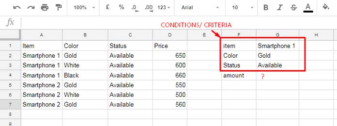
The sample data consists of smartphone models in column A, their colors in column B, availability status in column C, and prices in column D.
Assume you want to find the price of “Smartphone 1” in “Gold” color, given that the status is “Available.”

Setup the Conditions
- Enter Smartphone 1 in cell G1.
- Enter the color Gold in cell G2.
- Enter the status Available in cell G3.
Steps
Step 1: Use MATCH with Multiple Conditions
Let’s first use the MATCH function with multiple conditions to locate the position where all the conditions match.
=ArrayFormula(MATCH(1, (A2:A=G1)*(B2:B=G2)*(C2:C=G3), 0))This follows the syntax:
MATCH(search_key, range, [search_type])- The search_key is
1because the range(A2:A=G1)*(B2:B=G2)*(C2:C=G3)evaluates to1(if all conditions are met) or0. - The search_type is
0since we need an exact match in an unsorted range.
The MATCH function returns the position of the row that satisfies all the conditions.
Step 2: Use INDEX to Retrieve the Value
Now, use the position returned by the MATCH function to retrieve the price from column D using the INDEX function.
The syntax is:
INDEX(reference, [row], [column])- The reference is
D2:D. - The row is the position returned by the MATCH formula.
The formula becomes:
=INDEX(D2:D, MATCH(1, (A2:A=G1)*(B2:B=G2)*(C2:C=G3), 0))Note:
When using INDEX, you don’t need to wrap the MATCH formula with the ARRAYFORMULA function.
The above is an example of a multiple-condition INDEX MATCH in Google Sheets.
Alternatives to Multiple-Condition Index Match
The FILTER function is a better alternative to using multiple-condition INDEX MATCH in Google Sheets.
In the following example, the FILTER formula provides a simpler solution compared to INDEX MATCH:
=FILTER(D2:D, A2:A=G1, B2:B=G2, C2:C=G3)This formula filters the range D2:D based on the conditions provided, returning the value(s) where all conditions evaluate to TRUE.
As a side note, the QUERY function can also replace multiple-condition INDEX MATCH. Here’s an example:
=QUERY(A1:D, "SELECT D WHERE A='"&G1&"' and B='"&G2&"' and C='"&G3&"' ")This formula queries the dataset in A1:D and retrieves values from column D that meet the conditions in columns A, B, and C.
Why Do People Still Use INDEX MATCH?
The answer is simple: it’s popular among Excel users. Older versions of Excel don’t include the FILTER function, so many tutorials are written from an Excel perspective. This makes INDEX MATCH widely recognized, especially among users who have switched from Excel to Google Sheets or use both applications simultaneously.


Hello Prashanth,
Your website is incredible. Thank you so much. It is a fantastic tool for learning Google Sheets.
My question is,
I have a very messy sheet used for scheduling. I want to find a client that could be anywhere in multiple columns.
In a new sheet, create a formula to search for a specific client and then return data associated with that client, such as cost, time, or income.
Is this possible to do with functions?
– URL (sample sheet) removed by admin –
Hi, Jack Christmann,
I’ve sent my request to get edit access to your sheet.
Further, in that sheet, show me your expected result.
That’ll possibly help me to understand the problem.
Thank you, Prashanth,
I granted you to access and expanded on what I was looking for in yellow.
I have tried messing around with different formulas to try to get the result I am looking for but have constantly failed.
I am wondering if what I am trying to do is even possible, or perhaps I need to change the way I have my data setup.
Thanks!
Hi, Jack Christmann,
Please check your sheet for my formula and a short note.
Can you provide more images and diagrams for this article? Seeing the code with the example spreadsheet is the most helpful for me.
Hi, Emily Stroud,
Based on your request I have updated the post to included a sample sheet.