Google Sheets has introduced a new feature that allows users to select multiple values in drop-down lists, known as multiple selection drop-downs.

This tutorial explains how to create multiple-selection-dependent drop-downs (drop-down chips) in Google Sheets.

Can you explain the difference between a drop-down, multiple-selection drop-down, dependent drop-down, and multiple-selection dependent drop-down in Google Sheets?

• Drop-down menu: A drop-down menu is a feature that allows you to select options from a predefined list in a cell. It uses data validation to limit input to specific options.
• Multiple Selection Drop-down Menu: Similar to a drop-down menu, but allows you to select more than one value in a cell. The selected values will be displayed as chips.
• Dependent Drop-down: A dependent drop-down consists of at least two drop-downs, where the options in the second menu depend on the selection made in the first menu. The items in the second menu change based on the items selected in the first menu.
• Multiple Selection Dependent Drop-down: Similar to a dependent drop-down, but with the added functionality of selecting multiple values in the menus.

Let’s proceed with the steps, starting with a sample data set.

Step 1: Prepare the Sample Data

We will use a table with three columns, labeled Fruits, Vegetables, and Grocery in cells A1, B1, and C1, respectively.

Below these headers, you will list the relevant items: fruit names in A2:A, vegetable names in B2:B, and grocery items in C2:C.

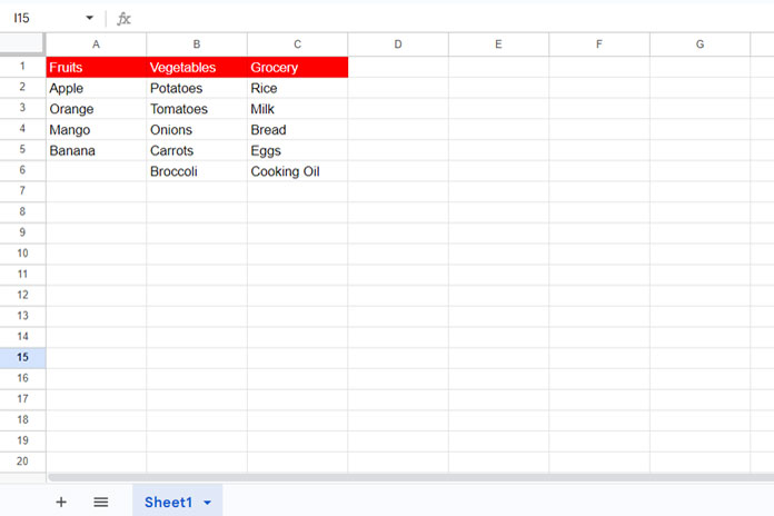
Assume the sheet containing this data is named Sheet1.

In Sheet2, we will create two drop-down chips (menus).

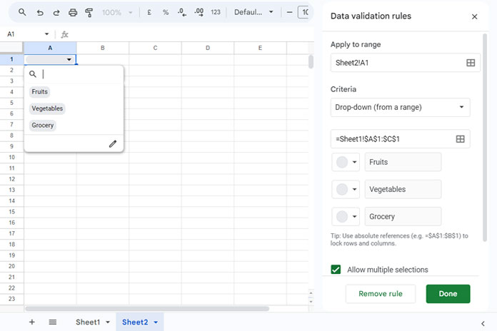
Step 2: Create the Multiple-Selection Drop-Down

Navigate to cell A1 in Sheet2, where we will create the multiple-selection drop-down chip.

1. Click Insert > Drop-down.
2. In the sidebar panel that opens, select Drop-down (from a range) under “Criteria.”
3. In the field below, enter Sheet1!A1:C1 to reference the column names from Sheet1.
4. Check the box that says “Allow Multiple Selections.”
5. Click Done to close the sidebar panel.

This will create a multiple-selection drop-down in cell A1.

Before we create the second drop-down that will depend on the multiple selections in the first drop-down, we need to add a formula in Sheet1. Let’s proceed to that step.

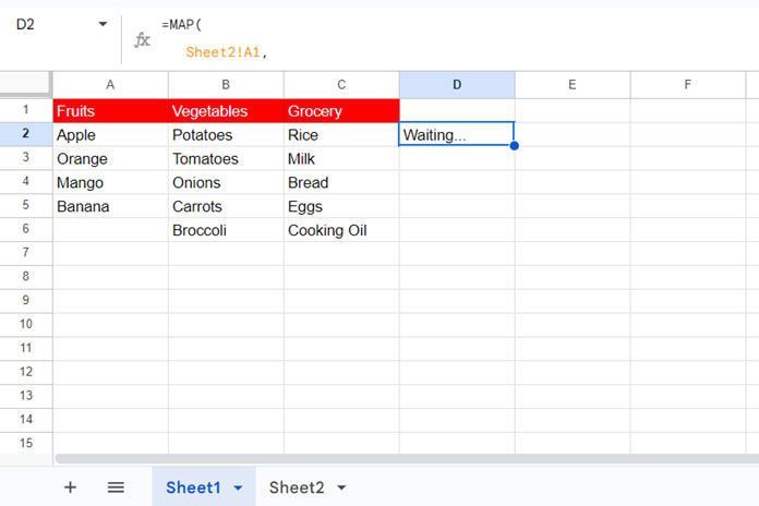
Step 3: Set Up the Helper Row for Multiple-Selection Dependent Drop-Downs

Enter the following formula in cell D2 in Sheet1:

=MAP(
   Sheet2!A1, 
   LAMBDA(
      choice, 
      IFNA(
         TOROW(
            FILTER(A2:C, XMATCH(A1:C1, SPLIT(choice, ", "))), 1
         ), "Waiting..."
      )
   )
)

Don’t worry about the complexity of the formula. If you follow the previous steps, this will work without any issues. For now, it will display the result “Waiting…”

Within the formula:

• Sheet2!A1 refers to the multiple selection drop-down chip in cell A1 in Sheet2.
• A1:C1 refers to the column names in the current sheet (Sheet1), to the left of the formula.
• A2:C refers to the data below the column names in the current sheet (Sheet1), to the left of the formula.

The formula filters the values in A2:C where A1:C1 matches the values selected in Sheet2!A1.

Step 4: Create the Multiple-Selection Dependent Drop-Down

Follow these steps:

1. Navigate to cell B1 in “Sheet2.”
2. Click Insert > Drop-down.
3. In the sidebar panel, select Drop-down (from a range) under “Criteria.”
4. Enter Sheet1!D2:2 in the field below.
5. Check the box for “Allow Multiple Selections.”
6. Click Done.

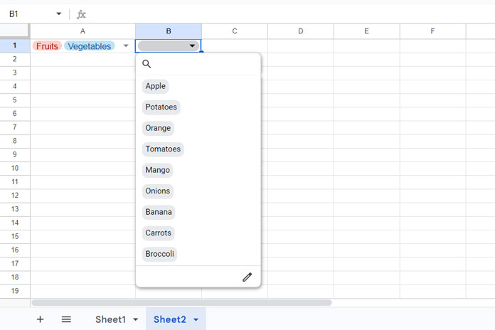
You have now created your first multiple-selection dependent drop-down list in Google Sheets. Let’s test it:

• Select “Fruits” in cell A1.
  Cell B1 will show the available fruits to select.
• Select “Fruits” and “Vegetables” in cell A1.
  Cell B1 will show the available fruits and vegetables.

Step 5: Customize for Multiple Row Support

If you want the drop-down list to work across multiple rows, simply copying and pasting the menus from A1 and B1 to the rows below will not work correctly.

To enable multiple-row support for the multiple-selection dependent drop-down list, follow these steps:

1. In the formula in “Sheet1,” replace Sheet2!A1 with Sheet2!A1:A.
2. Navigate to cell B1 in “Sheet2” and click Insert > Drop-down again.
3. Replace the reference =Sheet1!$D$2:$2 (absolute reference) in the sidebar panel with =Sheet1!D2:D (relative reference).
4. Click Done.

Now, copy the drop-down chips from A1:B1 and paste them down as far as you need. Then, select the range A1:B and press Delete to clear any previously selected values. That’s all!

Here is my template for you to test the functionality:

Sample Sheet Download

Additional Notes

If you select “Fruits” and “Vegetables” in cell A1, the multiple-selection dependent drop-down in cell B1 will list all items under these categories. Once you select values in cell B1, any changes made to A1 will not automatically update B1. To refresh the options in B1, you need to delete its current values and reselect from A1.

The formula uses a LAMBDA function to support multiple rows for the multiple-selection dependent drop-down list. Be aware that LAMBDA functions can experience performance issues with very large datasets.

Resources

• Highlighting Incorrect Dependent Text in Google Sheets
• Group-Wise Dependent Serial Numbering in Google Sheets
• Distinct Values in Drop-Down List in Google Sheets
• Getting an All Selection Option in a Drop-down in Google Sheets
• Create a Drop-Down to Filter Data From Rows and Columns
• Create a Drop-Down Menu From Multiple Ranges in Google Sheets
• Relative Reference in Drop-Down Menu in Google Sheets