


")


")

")
")
 in Excel & Google Sheets")


If your data is arranged in vertical groups, such as survey responses or employee records listed in stacked rows, you can transpose each set of rows into columns for easier analysis. In this tutorial, I’ll show you how to move each set of rows to columns in Google Sheets using two methods:
Transpose Each Set of Rows into Columns Using WRAPCOLS
The WRAPCOLS function is ideal for transforming vertical row groups into columns. It wraps values from a single column into multiple columns based on a specified group size.
Use Case Example:
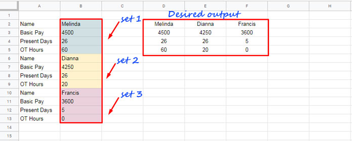
Imagine you have employee data in column B with repeating groups of 4 rows for each employee (e.g., Name, Basic Pay, Present Days, OT Hours). You want to convert that vertical data into a horizontal table where each group forms a column.
Formula:
=WRAPCOLS(B2:B13, 4, "")Formula Breakdown:
B2:B13– the range of stacked values.4– the number of rows in each group.""– optional padding if the data doesn’t divide evenly.
Syntax:
WRAPCOLS(range, wrap_count, [pad_with])Handling Dynamic or Expanding Data
If your dataset grows over time, use an open-ended range:
=WRAPCOLS(B2:B, 4, "")However, this can result in a #REF! error if data exists in cells where the formula is expected to spill results.
To fix this, use a dynamic range that automatically adjusts to the last non-blank cell:
=WRAPCOLS(INDEX(B2:XLOOKUP(TRUE, B2:B<>"", B2:B, ,0, -1)), 4, "")Optional: Remove All Empty Cells Before Wrapping
If you want to eliminate all empty cells before using WRAPCOLS, use TOCOL:
=WRAPCOLS(TOCOL(B2:B, 3), 4, "")Note: This removes all blanks, not just trailing ones. That means the row groupings may become misaligned, especially if blanks are meaningful.
VLOOKUP Trick to Transpose Each Set of Rows into Columns (Legacy Method)
Before WRAPCOLS was introduced, we used a clever VLOOKUP trick to transpose each set of rows into columns. Here’s how it works:
=ARRAYFORMULA(
  VLOOKUP(
    TRANSPOSE(SEQUENCE(ROUNDUP(ROWS(B2:B13)/4), 4)),
    {SEQUENCE(ROWS(B2:B13)), B2:B13},
    2,
    FALSE
  )
)
How This Works:
SEQUENCE(ROUNDUP(ROWS(B2:B13)/4), 4) – creates a vertical matrix of sequential numbers filled column-wise, e.g.:
| 1 | 2 | 3 | 4 |
| 5 | 6 | 7 | 8 |
| 9 | 10 | 11 | 12 |
TRANSPOSE(...) – flips the matrix to organize the sequence numbers in row-wise groups:
| 1 | 5 | 9 |
| 2 | 6 | 10 |
| 3 | 7 | 11 |
| 4 | 8 | 12 |
{SEQUENCE(...), B2:B13} – creates a lookup table where:
- Column 1 = sequence numbers (1 to 12)
- Column 2 = corresponding data in B2:B13
VLOOKUP(..., 2, FALSE) – uses the transposed sequence numbers to look up and return matching values from B2:B13, effectively transposing each set of 4 rows into a column-aligned format.
Just like with WRAPCOLS, you can adapt this formula to use a dynamic range:
=ARRAYFORMULA(
  VLOOKUP(
    TRANSPOSE(SEQUENCE(ROUNDUP(ROWS(B2:XLOOKUP(TRUE, B2:B<>"", B2:B, ,0, -1))/4), 4)),
    {SEQUENCE(ROWS(B2:XLOOKUP(TRUE, B2:B<>"", B2:B, ,0, -1))), B2:XLOOKUP(TRUE, B2:B<>"", B2:B, ,0, -1)},
    2,
    FALSE
  )
)
Summary
You’ve now learned how to move each set of rows to columns in Google Sheets using both a modern and legacy method. Whether you’re working with survey responses, employee records, or any stacked dataset, these techniques can help you transpose each set of rows into columns cleanly and dynamically.
Hello! I am looking to transpose every x number of cells. I cannot seem to figure it out. Could you please assist?
This may help.
=WRAPROWS(FILTER(A1:A,NOT(A1:A="")),5)In this case, 5 represents the variable n.
This worked perfectly! Thank you!!!
Hello! My case is similar to Alex, but if I wanted more columns, what do I do?
Example:
This
A|B|C|D|E|F|G|H
I|J|K|L|M|N|O|P
to this.
A|B|C|D
E|F|G|H
I|J|K|L
M|N|O|P
Hi, Poka,
There are much simpler ways now! Try this formula that uses TOCOL and WRAPROWS functions.
=wraprows(tocol(A1:H2),4)On Sheet1, I have 3 columns and 800 rows of data, formatted like so:
————–
A1 | B1 | C1
————–
A2 | B2 | C2
————–
A3 | B3 | C3
————–
etc.
On Sheet2, I would like the data to transpose into the following format:
———
A1 | B1
———
C1 |
———
A2 | B2
———
C2 |
———
A3 | B3
———
C3 |
———
etc.
What I want to do is figure out the formula for the first two rows in Sheet2, copy them, and paste them all the way down so that I’ll have all 800 rows of data from Sheet1 transposed over in the second format. Is this possible? Let me know if I need to reword my explanation.
Hi, Alex,
I have tested it with data in the range A2:C in Sheet1.
Here is the formula for Sheet2 that does the job.
=ArrayFormula(query({{row(Sheet1!A2:A),Sheet1!A2:B};{row(Sheet1!A2:A),Sheet1!C2:C,iferror(Sheet1!C2:C/0)}},
"Select Col2,Col3 where Col2 is not null order by Col1"))
Can you explain how to transpose a vertical range to horizontal but add seven blank spaces in between each transposed value?
Hi, Jackson,
First, insert blank rows using a formula and then transpose.
The below formula is for the range A2:A.
=transpose(ArrayFormula(iferror(vlookup(array_constrain(row(A8:A),
COUNTA(A2:A)*8-7,1),{if(len(A2:A),row(A1:A)*8,),A2:A},2,false)," "))
)
Try it in B1 after emptying B1:1