


")


")

")
")
 in Excel & Google Sheets")


We typically use multiple SUMIF functions to return individual totals for multiple columns based on a criteria column. Recently, you can automate this process with the BYCOL function in conjunction with SUMIF. Other alternatives include DSUM, which requires structured data, and MMULT. This tutorial explains how to use the MMULT function as an alternative to the SUMIF function for calculating conditional totals in Google Sheets.
Let’s begin with the regular SUM function and its MMULT counterpart.
Using MMULT as a Replacement for SUM in Google Sheets
Assume you have items in A1:A7 and corresponding sales quantities from January to March in B1:D7.
You can use the following SUM formula in cell B8 and drag it to D8 to get the total for each column:
=SUM(B2:B7)If you don’t want to drag the SUM formula across, you can replace it with the following MMULT formula:
=MMULT(SEQUENCE(1, ROWS(A2:A7), 1, 0), B2:D7)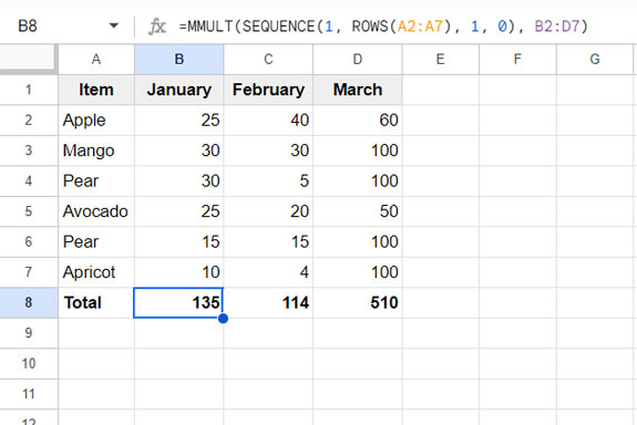
In this, matrix 1 is SEQUENCE(1, ROWS(A2:A7), 1, 0), which returns 1’s horizontally equal to the number of rows in the range. Matrix 2 is B2:D7.
The result of matrix multiplication will be the individual total for each column.
Now, consider the following SUMIF formula:
=SUMIF($A$2:$A$7, "Pear", B2:B7)If you enter it in cell B9 and drag it to D9, it will return the total quantities for the item “Pear” in each month.
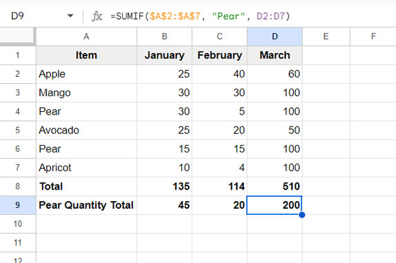
You can replace the above SUMIF formula with an MMULT formula for conditional totals across the row. Let’s dive into the details.
MMULT as an Alternative to SUMIF for Conditional Totals: Single Criterion
When applying a condition, you need to modify the criteria column (A2:A7) used in the SUMIF function.
In the previous regular MMULT example, the matrix 1 was SEQUENCE(1, ROWS(A2:A7), 1, 0), which returned the array {1, 1, 1, 1, 1, 1}.
To apply the condition, you replace the value 1 with 0 wherever the criterion “Pear” doesn’t match in A2:A7.
This formula does that effectively: =ArrayFormula(TOROW(N(A2:A7="Pear"))).
A2:A7="Pear"returns an array of TRUE or FALSE, where TRUE means the criterion matches.- N function converts TRUE to 1 and FALSE to 0.
- TOROW changes the array from vertical to horizontal orientation.
Now, the matrix will look like this: {0, 0, 1, 0, 1, 0}.
The MMULT formula to replace SUMIF is:
=ArrayFormula(MMULT(TOROW(N(A2:A7="Pear")), B2:D7))MMULT as an Alternative to SUMIF for Conditional Totals: Multiple Criteria
In the above example, we applied only one condition. Unlike SUMIF, which is dedicated to utilizing a single condition, MMULT allows us to specify multiple conditions.
To get the total for “Pear” and “Apple,” specify matrix 1 as follows:
=ARRAYFORMULA(TOROW((A2:A7="Pear")+(A2:A7="Apple")))The N function is not required here since the addition converts TRUE to 1 and FALSE to 0.
Thus, the MMULT formula with multiple conditions will be:
=ArrayFormula(MMULT(TOROW((A2:A7="Pear")+(A2:A7="Apple")), B2:D7))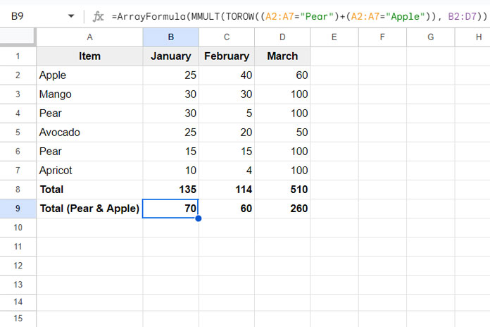
That’s really great, thanks!
I’ve been searching for two days.
Is it much more efficient than expending a traditional SUMIF in terms of calculation time?
Also, would it be possible to do the same to get the average and the standard deviation?
Hi, Grange Romain,
Regarding efficiency, if the data is small, it won’t make much difference. Otherwise, I would prefer the SUMIF over the MMULT.
There is a much more efficient formula for a larger dataset. It is by using the DSUM database function.
For that, we should make the data structured. Please refer to my sample data screenshot. In that, I have merged a few cells in the title. Remove them.
So the field labels “Name” should be in A4 and “Unit Rate” in B4.
Then you can use the below DSUM instead of the MMULT.
=ArrayFormula(dsum(A4:H10,{3,4,5,6,7,8},{"Name";"Peer"}))For standard deviation, replace DSUM in the above formula with the DSTDEV function.
=ArrayFormula(dstdev(A4:H10,{3,4,5,6,7,8},{"Name";"Peer"}))For average, replace DSUM with DAVERAGE.
=ArrayFormula(daverage(A4:H10,{3,4,5,6,7,8},{"Name";"Peer"}))It was helpful!
I hadn’t been able to expand my row for days. I tried counts, filters, and sums in every way I could think.
It was an elegant solution, though!