


")


")

")
")
 in Excel & Google Sheets")


The MATCH function in Google Sheets returns the relative position of a value within a list or range. The relative position refers to where an item appears inside the specified range, not its actual row or column number in the sheet.
Quick Answer
MATCH searches for a value and returns its position in a list. It is commonly used with INDEX to look up related values dynamically—MATCH returns the relative position, while INDEX returns the value at that position.
What Is the MATCH Function Used For in Google Sheets?
The MATCH function in Google Sheets is used to:
- Find the position of a value in a list
- Return row numbers (vertical search)
- Return column numbers (horizontal search)
- Build dynamic lookup formulas with INDEX or FILTER
Tip: When combined with INDEX, MATCH becomes a powerful alternative to VLOOKUP and HLOOKUP.
MATCH Function Syntax
MATCH(search_key, range, [search_type])
Arguments Explained
- search_key
The value you want to find (text, number, or date). - range
A one-dimensional range to search (single row or column). - search_type (optional)
Controls how the MATCH function finds the result.
If omitted, the default value is1.
| Value | When to Use | Behavior |
|---|---|---|
0 | Unsorted range | Exact match |
1 | Sorted ascending | Largest value ≤ search_key |
-1 | Sorted descending | Smallest value ≥ search_key |
⚠️ Common mistake: Using 1, -1, or omitting the last argument on an unsorted range can return incorrect results.
MATCH Function in an Unsorted Range (Exact Match)
This is the most common use case for the MATCH function in Google Sheets. Always use 0 for exact matching.
Example: Text Search
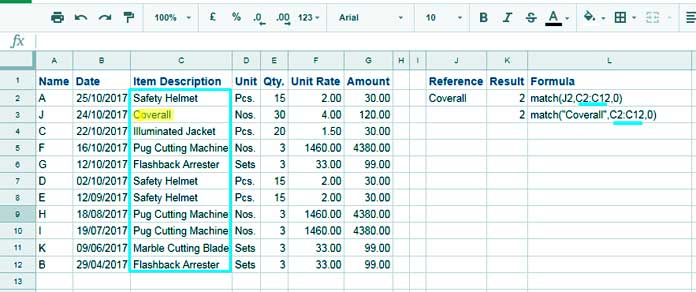
To find the position of “Coverall” in C2:C12:
=MATCH("Coverall", C2:C12, 0)
Or using a cell reference:
=MATCH(J2, C2:C12, 0)
Result: 2 (because “Coverall” appears in cell C3)
Notes
- Returns the first match if duplicates exist
- Use
C:Cinstead ofC2:C12to get the row number - Returns
#N/Aif no match is found
Handling #N/A Errors
You can use the IFNA function to handle #N/A errors and return an empty cell or a custom value instead.
=IFNA(MATCH(J2, C2:C12, 0))
If you want to show a custom message, you can use:
=IFNA(MATCH(J2, C2:C12, 0), "Not found")MATCH with Numbers
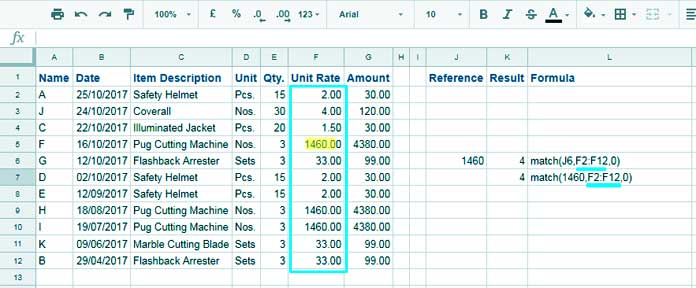
To find the position of 1460 in F2:F12:
=MATCH(1460, F2:F12, 0)
Or:
=MATCH(J6, F2:F12, 0)
MATCH with Dates in Google Sheets
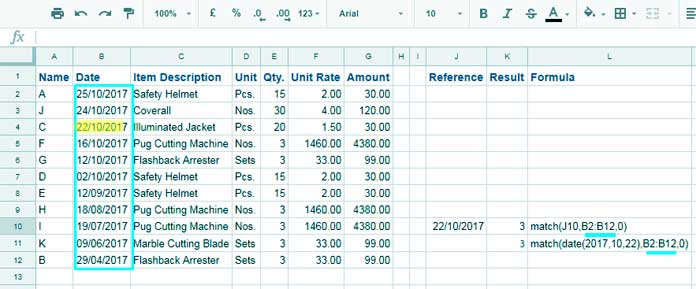
If the search key is a cell reference, no extra steps are needed:
=MATCH(J10, B2:B12, 0)
If the date is hard-coded, always use the DATE function:
=MATCH(DATE(2017,10,22), B2:B12, 0)
This avoids date-format mismatches.
MATCH Function in a Sorted Range
Ascending Order Example
Range: 1, 5, 6, 10, 15
Search key: 8
=MATCH(8, A1:A5, 1)
Result: 3
(Largest value ≤ 8 is 6)
Descending Order Example
Range: 15, 10, 6, 5, 1
Search key: 8
=MATCH(8, A1:A5, -1)
Result: 2
(Smallest value ≥ 8 is 10)
MATCH with FILTER in Google Sheets
The MATCH function can return multiple results when used with ARRAYFORMULA.
=ARRAYFORMULA(MATCH(A1:A7, F1:F2, 0))
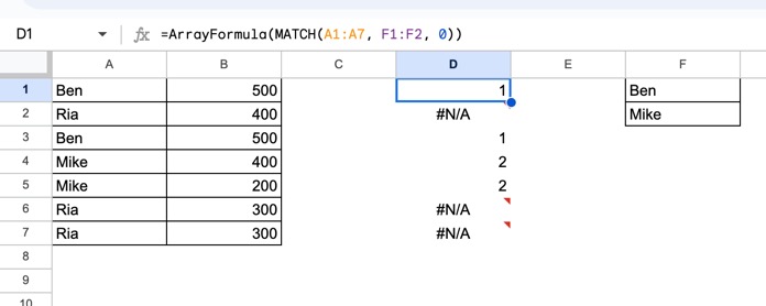
To filter corresponding values:
=FILTER(B1:B7, MATCH(A1:A7, F1:F2, 0))
This returns only rows where matches exist.
Using MATCH Inside INDEX (Most Important Use Case)
The most practical use of the MATCH function in Google Sheets is inside INDEX.
Example Table
| Item | Price |
|---|---|
| Apple | 5 |
| Orange | 4.5 |
| Mango | 5.25 |
| Banana | 3.25 |
| Pineapple | 4.75 |
| Grape | 6 |
Formula:
=INDEX(B1:B6, MATCH("Grape", A1:A6, 0))
Result: 6
This creates a dynamic lookup that doesn’t break when rows are inserted or deleted.
Related: Index-Match: Better Alternative to Vlookup and Hlookup in Google Sheets
Horizontal MATCH Example
If values are in C1:Q1:
=MATCH("Sales", C1:Q1, 0)
To return the column number, use:
=MATCH("Sales", 1:1, 0)
MATCH vs XMATCH in Google Sheets
Google Sheets now includes XMATCH, which adds several advanced capabilities:
- Supports reverse searches
- Supports wildcards
- Uses binary search for faster lookups on sorted data
- Replaces many advanced MATCH use cases
However, the MATCH function in Google Sheets is still widely used because it is simpler, faster, and sufficient for most lookup scenarios.
Final Thoughts
The MATCH function in Google Sheets is essential for:
- Exact lookups
- Dynamic row and column detection
- Advanced formulas using INDEX and FILTER
If you master MATCH, you unlock the real power of spreadsheet automation.
Hi Prashanth 🙂
I would like to ask you regarding MATCH function.
If I have 2 tables with the same name and column such as :-
TABLE A : [Name, Age, Address] TABLE B : [Name, Age, Address]
I want to make another table (TABLE C-with the same column & name) , to combine both data in the new table. But, if the row in TABLE A is match with TABLE B, it will take only one row instead of taking both rows (if it takes both, the data is redundant).
Is it possible to use MATCH or any other formula for it?
Thank you so much 🙂
https://infoinspired.com/google-docs/spreadsheet/merge-two-tables-in-google-sheets/