There are many functions to look up a value in a table in Google Sheets. Among them, VLOOKUP, HLOOKUP, and LOOKUP are the most popular. To correctly choose between these functions, you must understand how they differ.
As a side note, Google Sheets offers an advanced lookup function called XLOOKUP. This function differs from the ones mentioned above, so we are not including it in our comparison.
Purpose
The purpose of the three lookup functions is the same: in a dataset (range), you can search for a keyword (search_key) and retrieve related information from other cells.
For example, I have a list with fruit names. I can search for the fruit name “Apple” in that list and return its price, quantity, or any other information present.
Which function you use depends on whether you want to look up the key in the first column, the first row, a specific row or column, or whether the data is sorted.
Among VLOOKUP, HLOOKUP, and LOOKUP, VLOOKUP is the most widely used because the data is typically arranged vertically and often unsorted. You will understand the distinctions between them as you go through the differences below.
How LOOKUP, VLOOKUP, and HLOOKUP Functions Differ in Google Sheets
First, let me point out the key differences between the LOOKUP, VLOOKUP, and HLOOKUP functions in Google Sheets. Then we’ll dive into examples to help you understand these differences in real-life use cases.
- VLOOKUP is for vertical lookup. It searches for the key in the first column of the range and returns the value from the specified column in the range, where the first column is numbered 1.
- HLOOKUP is for horizontal lookup. It searches for the key in the first row of the range and returns the value from the specified row, where the first row in the range is numbered 1.
There are two types of use cases for LOOKUP:
- LOOKUP searches the first row if the range is wider and returns the result from the last row. If the range is taller, it searches the first column and returns the result from the last column. If the number of rows and columns are equal in the range, it will perform a vertical lookup.
- Alternatively, you can specify the row or column to search for the key, as well as the row or column to return the result. This involves the search key, search range (row or column), and result range (row or column).
While VLOOKUP and HLOOKUP can work with both sorted and unsorted data, LOOKUP works only with sorted data.
In sorted data, when the search key is not found, all these lookup functions will perform an approximate match of the search key. In that case, the item used in the lookup will be the value that is immediately smaller than the search key in the provided range.
You can specify multiple result column indexes, such as {2, 3, 4}, in VLOOKUP and HLOOKUP, and enter them as an array formula to return multiple values. In contrast, LOOKUP doesn’t support this.
All these functions support wildcards for partial matches.
The above are the key LOOKUP, VLOOKUP, and HLOOKUP differences in Google Sheets. Now, let’s look at a few examples to understand them better.
Examples
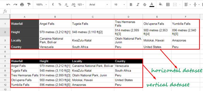
In the following example, I have two tables: One in the range A1:F4 and another in the range A7:D12. The first table is a horizontal dataset, and the second one is a vertical dataset. They contain the same data—waterfall details—but with different orientations.

You can get my sample sheet by clicking the button below and follow the examples in your copy.
In the first table, waterfall names are in the first row, and in the second table, they’re in the first column. We’ll search for a particular waterfall name in these tables using LOOKUP, VLOOKUP, and HLOOKUP to understand their differences.
First, we will start with VLOOKUP and HLOOKUP since the data is not sorted (the waterfall names are not in order).
VLOOKUP:
In the second table, we can use the following VLOOKUP formula to search for “Angel Falls” in the first column and return the country from the 4th column:
=VLOOKUP("Angel Falls", A7:D12, 4, FALSE)It follows the syntax:
VLOOKUP(search_key, range, index, [is_sorted])The last argument, is_sorted, is FALSE because the data is not sorted.
HLOOKUP:
In the first table, use the following HLOOKUP to search for “Angel Falls” in the first row and return the country from the fourth row:
=HLOOKUP("Angel Falls", A1:F4, 4, FALSE)The syntax is:
HLOOKUP(search_key, range, index, [is_sorted])Again, the fourth argument is FALSE because the data is unsorted.
LOOKUP:
LOOKUP is unsupported in this case since the tables are not sorted.
Using LOOKUP, VLOOKUP, and HLOOKUP in Sorted Tables to See the Differences
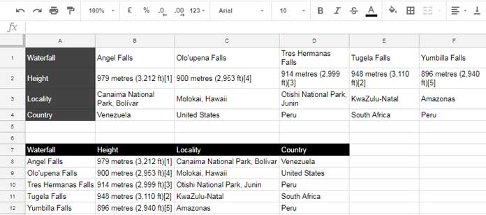
Below, you will see the same tables as above, but now the system has sorted them. The waterfall names are in sorted order in both the horizontal and vertical datasets.

In these sorted tables, you can use the same VLOOKUP and HLOOKUP formulas. The results will be the same.
Now let’s look at examples using LOOKUP to see how this function differs from the other two.
You can use the following formula in the first table to look up “Angel Falls” in the first row and return the country from the last row:
=LOOKUP("Angel Falls", A1:F4)For the vertical dataset, you can use the following formula:
=LOOKUP("Angel Falls", A7:D12)LOOKUP searches the first column for the key and returns the result from the last column.
The formula automatically identifies the data’s arrangement—whether horizontal or vertical—and searches the first row or column accordingly.
These two formulas follow the syntax:
LOOKUP(search_key, search_result_array)Now, see the below two formulas:
=LOOKUP("Angel Falls", A1:F1, A4:F4) // searches the row range A1:F1 and returns the result from the row range A4:F4
=LOOKUP("Angel Falls", A7:A12, D7:D12) // searches the column range A7:A12 and returns the result from the column range D7:D12
These two formulas follow the syntax:
LOOKUP(search_key, search_range, result_range)Conclusion
We’ve covered the key LOOKUP, VLOOKUP, and HLOOKUP differences in Google Sheets.
Additionally, advanced users can overcome the issue associated with LOOKUP’s sorted data requirement by using the SORT function with the range.
Unlike LOOKUP, VLOOKUP and HLOOKUP can return multiple values. For example, you can specify multiple index numbers as follows:
=ArrayFormula(VLOOKUP("Angel Falls", A7:D12, {3, 4}, FALSE))// returns locality and country=ArrayFormula(HLOOKUP("Angel Falls", A1:F4, {3, 4}, FALSE))// returns locality and country
XLOOKUP is a more modern function that combines most of the features of these functions, along with additional capabilities. However, it does not include all features, as it lacks the two-argument approach used by LOOKUP, which involves search_key and search_result_array.
That concludes the key differences between LOOKUP, VLOOKUP, and HLOOKUP in Google Sheets.


