


")


")

")
")
 in Excel & Google Sheets")


Looking up the last occurrence of a partial match in Google Sheets can be useful in various real-world scenarios, such as:
- Tracking the last purchase of a customer based on a partial name match.
- Finding the last login of a user based on a partial username match.
- Identifying the last order of a product when product names include variations (e.g., “Apple Juice,” “Apple Cider”).
In this tutorial, you’ll learn how to use XLOOKUP to find the last occurrence of a partially matching keyword. We’ll explore case-sensitive, case-insensitive, and exact word match methods.
Case-Insensitive Formulas for Finding the Last Partial Match
Basic Case-Insensitive XLOOKUP:
=XLOOKUP("*search_key*", lookup_range, result_range, , 2, -1)With Word Boundary (Exact Match within a String):
=ArrayFormula(XLOOKUP(TRUE, REGEXMATCH(lookup_range, "(?i)\bsearch_key\b"), result_range, , 0, -1))Case-Sensitive Formulas for Finding the Last Partial Match
Basic Case-Sensitive XLOOKUP:
=ArrayFormula(XLOOKUP(TRUE, REGEXMATCH(lookup_range, "search_key"), result_range, , 0, -1))With Word Boundary (Exact Match within a String):
=ArrayFormula(XLOOKUP(TRUE, REGEXMATCH(lookup_range, "\bsearch_key\b"), result_range, , 0, -1))Example 1: Case-Insensitive Lookup for the Last Partial Match
Consider the following product sales data:
| Item | Qty |
| Apple Juice | 2 |
| Orange Soda | 4 |
| Apple Pie | 1 |
| Grape Juice | 5 |
| Apple Cider | 6 |
| Mango Shake | 8 |
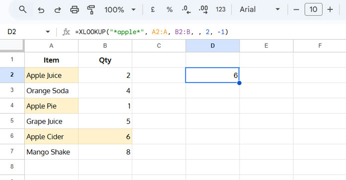
If we want to find the quantity of the last occurrence of “Apple”, the formula would be:
=XLOOKUP("*apple*", A2:A, B2:B, , 2, -1)This formula searches from bottom to top and finds “Apple Cider” (Qty: 6).
📝 Note: Repalce "*apple*" with "*"&D1&"*" when the search key is in cell D1.
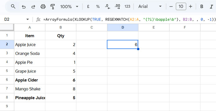
Potential Issue: What if “Pineapple Juice” is added as the last row?
Pineapple Juice | 5
The formula will incorrectly return 5, as “apple” appears in “Pineapple” too.
Fix: Use an exact word match to exclude such cases:
=ArrayFormula(XLOOKUP(TRUE, REGEXMATCH(A2:A, "(?i)\bapple\b"), B2:B, , 0, -1))Now, it correctly returns 6 (Apple Cider) instead of 5 (Pineapple Juice).
📝 Note: Repalce "(?i)\bapple\b" with "(?i)\b"&D1&"\b" when the search key is in cell D1.
Why REGEXMATCH?
The REGEXMATCH function checks if a text contains a specific pattern. Here, (?i)\bapple\b ensures a case-insensitive match ((?i)) and enforces word boundaries (\b) so that “Apple” is matched as a standalone word, not as part of “Pineapple.”
Example 2: Case-Sensitive Lookup for the Last Partial Match
Consider a login record:
| Username | Last Login |
| John_91 | 01/02/2025 |
| jack001 | 02/02/2025 |
| Jenny | 03/02/2025 |
| miKe1 | 04/02/2025 |
| john_86 | 05/02/2025 |
| Rose_86 | 06/02/2025 |
| john_86 | 07/02/2025 |
| John_91 | 08/02/2025 |
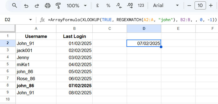
To find the last login date of “john” (case-sensitive):
=ArrayFormula(XLOOKUP(TRUE, REGEXMATCH(A2:A, "john"), B2:B, , 0, -1))Returns 07/02/2025 (last occurrence of “john”).
📝 Note: Repalce "john" with D1 when the search key is in cell D1.
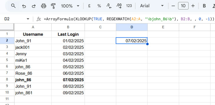
Potential Issue: If “john_861” is added as the last row:
john_861 | 09/02/2025
The formula will return 09/02/2025, which is incorrect if we wanted exact “john_86”.
Fix: Apply a word boundary to exclude extra characters:
=ArrayFormula(XLOOKUP(TRUE, REGEXMATCH(A2:A, "\bjohn_86\b"), B2:B, , 0, -1))Now, it correctly returns 07/02/2025.
📝 Note: Repalce "\bjohn_86\b" with "\b"&D1&"\b" when the search key is in cell D1.
When to Use Case-Sensitive Lookup?
Case-sensitive lookups are useful when dealing with:
- Usernames (e.g., “John_86” ≠ “john_86”).
- Item codes (e.g., “ABC12” ≠ “abc12”).
- Product IDs where letter case matters.
Key Takeaways
- Use XLOOKUP with wildcards (
*search_key*) for flexible, case-insensitive partial matches. - Use REGEXMATCH with word boundaries (
(?i)\bsearch_key\b) when you need an exact word match. - Opt for case-sensitive formulas when working with usernames, item codes, or situations where letter case matters.
How would I do multiple
find()in thelookup()?For example, let’s say column C is a list of reasons they were absent (sick, vacation, etc). I want to find the last occurrence of “Samuel Barnes” in column A and “sick” in column C and return the date from column B.
Hi, Dan,
Good question 🙂
For that, you can use this formula.
=ArrayFormula(lookup(1,(find("Samuel Barnes",A2:A)+find("Sick",C2:C))/(find("Samuel Barnes",A2:A)+find("Sick",C2:C)),B2:B))See this similar tutorial – Lookup to Find the Last Occurrence of Multiple Criteria in Google Sheets.
For case insensitive, if you want, replace the function FIND with SEARCH.