")
")


")


")

")
")
 in Excel & Google Sheets")


The Google Sheets QUERY function allows you to efficiently manipulate data for a wide range of use cases. It helps extract meaningful information from large or complex datasets and makes it easier to build reports, summaries, charts, and more.
One of the key strengths of the QUERY function is that it uses the Google Visualization API Query language, which enables powerful data operations such as filtering, grouping, sorting, pivoting, and aggregation—all within a single formula.
In short, the QUERY function is the most powerful data-manipulation tool in Google Sheets. This tutorial covers everything you need to understand and confidently use the QUERY function through clear explanations and practical examples.
Google Sheets QUERY Function Syntax (With Examples)
Let’s begin with the syntax of the QUERY function in Google Sheets.
Unlike many other functions, the QUERY function is not easy to understand by simply looking at its arguments. Don’t worry—its logic becomes much clearer once you work through examples step by step, which is exactly what this guide focuses on.
Syntax
QUERY(data, query, [headers])
Arguments
data
The range of cells (table) on which the query is performed. For accurate results, each column should contain a single data type.
What is mixed-type data?
For example, if column A contains item codes such as 1111, 1112, 1113, and so on, all values should be formatted consistently—either as numbers or as text, but not a mix of both.
In general:
- A numeric column should contain only numbers
- A date column should contain only dates
- A text column should contain only text values
query
The query statement you want to run. It must be enclosed in double quotes, or you can store the query text in a cell and reference that cell in the formula.
headers
The number of header rows in the source data. Most datasets have either one header row or none.
If this argument is omitted or set to -1, Google Sheets automatically guesses the number of header rows based on the data.
Example
=QUERY(A1:F1000, "SELECT A, C", 1)
In this formula:
A1:F1000is the data range"SELECT A, C"is the query1indicates that the first row contains headers
The result returns only columns A and C from the dataset.
To truly master the Google Sheets QUERY function, the key is understanding the query argument, which is where most of the power—and complexity—lies. The following sections focus heavily on breaking this down with practical examples.
How the QUERY String Works (Simplifying the Query Argument)
When you read a QUERY formula written by someone else, the most confusing part is usually the query string enclosed in quotation marks. This section contains clauses (keywords), data-manipulation logic, and other language elements that can look intimidating at first.
Trying to learn every clause and function in a single tutorial isn’t practical. Instead, this guide focuses on helping you understand the essential data-manipulation techniques used in the Google Sheets QUERY function, step by step.
As you progress, I’ll also point you to more advanced tutorials on this blog so you can gradually master one of the most powerful functions available in Google Sheets.
Let’s get started.
Sample Dataset Used in All QUERY Function Examples
We’ll use a sample dataset arranged across six columns and sixteen rows, located in the range A1:F16 on the Sheet1 tab.
The header row (A1:F1) contains the following field names:
- Name
- DOB
- Age Group
- Gender
- Date of Joining
- Age
You can get a copy of the complete dataset by clicking the button below.
All QUERY function examples in this guide are based on this sample sheet. Before proceeding, it’s a good idea to scroll up and review the QUERY function syntax once more.
As a reminder, the QUERY function has three arguments:
- data
- query
- headers
Based on this sample sheet:
- The data argument can be
A1:F(open range) orA1:F16(closed range) - The headers argument is
1, since the first row contains column labels
In the following sections, we’ll focus primarily on the query argument, where most of the QUERY function’s power lies.
SELECT Clause in Google Sheets QUERY (With Examples)
This section explains how to select columns in the QUERY function using the SELECT clause.
Basic SELECT Examples
Using the sample dataset (six columns in Sheet1!A1:F16), you can select and rearrange columns with the SELECT clause in the Google Sheets QUERY function.
=QUERY(Sheet1!A1:F16, "SELECT A, B, F, C, D, E", 1)
The formula above returns the selected columns in a different order.
=QUERY(Sheet1!A1:F16, "SELECT A, E", 1)
This formula returns only columns A and E.
If you replace "SELECT A, E" with "SELECT *", the QUERY function returns all columns from the source table in their original order.
Returning All Columns Without a SELECT Clause
An alternative way to return all columns in their original order is to omit the query argument entirely:
=QUERY(Sheet1!A1:F16,, 1)
Here, only the data and headers arguments are specified.
If you specify 16 instead of 1 for the headers argument, the formula returns a 1-row × 6-column result, treating all rows as headers.
For more details on this behavior, see: The Flexible Array Formula to Join Columns in Google Sheets.
Using Arithmetic, Scalar, and Aggregation Functions in SELECT
So far, we’ve selected existing columns without modifying their values. Let’s now look at how to process column data using functions and operators inside the SELECT clause.
Scalar Function: YEAR() in the SELECT Clause
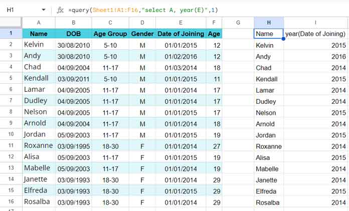
=QUERY(Sheet1!A1:F16, "SELECT A, YEAR(E)", 1)
This formula returns:
- Column A (Name)
- The year of joining, extracted from column E (Date of Joining)
Common Scalar Functions Used in QUERY
| Function | Purpose |
|---|---|
year() | Extracts the year from a date or datetime |
month() | Returns month (0–11) from a date or datetime |
day() | Returns day of the month |
hour() | Returns hour from a datetime |
minute() | Returns minutes from a datetime |
second() | Returns seconds from a datetime |
millisecond() | Returns milliseconds |
quarter() | Returns quarter of the year |
dayOfWeek() | Returns day of week (Sun = 1, Sat = 7) |
now() | Returns current datetime (GMT timezone). Typically used in the WHERE clause, not SELECT. |
dateDiff() | Returns difference between two dates (days) |
toDate() | Converts a value to a date |
upper() | Converts text to uppercase |
lower() | Converts text to lowercase |
Further reading on scalar functions in QUERY:
- How to Use the
DATEDIFF()Function in Google Sheets QUERY - How to Use the
toDate()Scalar Function in Google Sheets QUERY - Use QUERY to Bulk Convert Text Cases in Google Sheets
Aggregation Function: AVG() in the SELECT Clause
To calculate the average age from column F:
=QUERY(Sheet1!A1:F16, "SELECT AVG(F)", 1)
This formula returns the average value of the Age column. If you want to perform additional calculations on QUERY results, see Sum, Multiply, Subtract & Divide in Google Sheets.
Combining Scalar Functions and Arithmetic Operators
To calculate age at the time of joining, subtract the year of birth from the year of joining:
=QUERY(Sheet1!A1:F16, "SELECT A, YEAR(E) - YEAR(B)", 1)
Note: This calculation considers only years, so the result may not be fully accurate due to month and day differences.
For more examples using +, -, *, and / inside QUERY, see How to Use Arithmetic Operators in Query in Google Sheets.
Column Identifiers Explained
In QUERY formulas, column identifiers are usually column letters such as A, B, C, … AA, AB, and so on.
When your data is a physical range like A1:F16, these standard column letters apply.
However, when QUERY works on the output of another formula (an expression), columns are identified as:
Col1→ first columnCol2→ second columnCol3→ third column
…and so on.
Inserting a Custom Column in SELECT
The following formula inserts a column containing hyphens between columns A and B:
=QUERY(Sheet1!A1:F16, "SELECT A, '-', B", 1)
This technique is useful when you want to add separators or placeholder values in the QUERY output.
Filtering Data Using QUERY WHERE Clause (Examples)
Above, we explored how to use the SELECT keyword in the Google Sheets QUERY function to choose specific columns.
Now let’s look at how to filter rows.
To filter rows based on conditions, you use the WHERE clause.
Common WHERE Clause Examples
In the WHERE clause, you use:
- Comparison operators (simple or complex), and/or
- Logical operators such as
AND,OR, andNOT
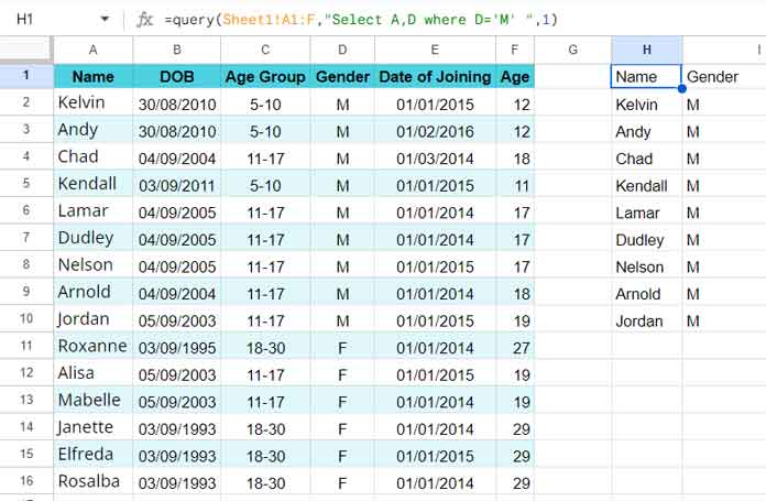
Using the sample data, the following formula filters rows where the gender is “M”:
=QUERY(Sheet1!A1:F, "SELECT A, D WHERE D = 'M'", 1)
The next formula filters names where the age is 12:
=QUERY(Sheet1!A1:F, "SELECT A WHERE F = 12", 1)
The following QUERY filters names whose date of joining is 01-01-2015:
=QUERY(Sheet1!A1:F, "SELECT A WHERE E = DATE '2015-01-01'", 1)
These examples serve two purposes:
- They demonstrate how to use the WHERE keyword in the QUERY function
- They show how to compare different literal types—text, numbers, and dates
Filtering Resources
For more comprehensive data-filtering techniques, refer to the tutorials below:
- Literals in Google Sheets QUERY – How to Use Them
- WHERE Clause in Google Sheets QUERY: Logical Conditions Explained (Hub)
- String Matching in Google Sheets QUERY (Hub)
Advanced Filtering Tips
In the examples above, filtering a Boolean (TRUE / FALSE) column is not shown because the sample dataset does not include one.
If column G contains Boolean values, you can filter it as follows:
WHERE G = TRUE
or
WHERE G = FALSE
Case Sensitivity in QUERY
String comparisons in the QUERY function are case-sensitive. To perform a case-insensitive match, use the UPPER() or LOWER() scalar functions.
Example:
=QUERY(Sheet1!A1:F, "SELECT A WHERE LOWER(D) = 'm'", 1)
Open vs. Closed Ranges in WHERE Filtering
You may have noticed that the examples above use an open range (Sheet1!A1:F) instead of a closed range (Sheet1!A1:F16).
This approach is useful when filtering conditions may remove blank rows from the result.
To explicitly exclude blank rows, you can use IS NOT NULL, as shown below:
=QUERY(Sheet1!A1:F, "SELECT A, E, F WHERE A IS NOT NULL", 1)
GROUP BY and Aggregation in Google Sheets QUERY (Examples)
So far, we’ve learned how to select columns and filter rows. This section focuses on how to group and aggregate data using the QUERY function in Google Sheets.
To do this, we use the GROUP BY clause. Like the WHERE clause, GROUP BY is a broad topic, so we’ll begin with a few basic examples before pointing you to more advanced resources.
Key Points About GROUP BY in QUERY
Keep the following rules in mind when using the GROUP BY clause:
- GROUP BY aggregates values across multiple rows
- One output row is created for each distinct group
- Results are automatically sorted by the grouping columns
- Every non-aggregated column in the SELECT clause must appear in the GROUP BY clause
- Aggregated columns (e.g.,
SUM(),COUNT(),AVG()) do not need to be grouped
- Aggregated columns (e.g.,
GROUP BY with SUM, COUNT, and AVG
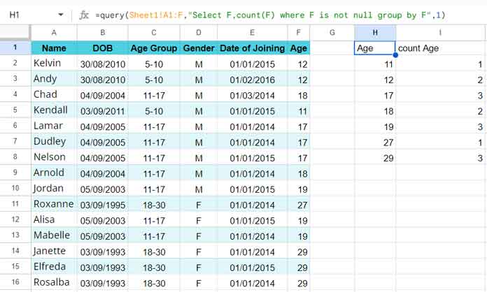
The following formula groups data by Age (column F) and returns the count for each age:
=QUERY(Sheet1!A1:F16, "SELECT F, COUNT(F) GROUP BY F", 1)
This formula groups data by Age and Date of Joining, then returns the count:
=QUERY(Sheet1!A1:F16, "SELECT F, E, COUNT(F) GROUP BY F, E", 1)
Using GROUP BY with Open Ranges
When using an open range, it’s important to exclude blank rows to avoid incorrect aggregation results.
=QUERY(Sheet1!A1:F, "SELECT F, COUNT(F) WHERE F IS NOT NULL GROUP BY F", 1)
Scalar Functions with GROUP BY
The following example groups data by the year of joining and returns the count:
=QUERY(A1:F, "SELECT YEAR(E), COUNT(E) WHERE E IS NOT NULL GROUP BY YEAR(E)", 1)
Here:
YEAR(E)extracts the year from the Date of Joining column- GROUP BY is applied to the computed value, not the original column
Arithmetic Operations with GROUP BY
You can also group by calculated expressions, as shown below:
=QUERY(A1:F, "SELECT YEAR(NOW()) - YEAR(E), COUNT(E) WHERE E IS NOT NULL GROUP BY YEAR(NOW()) - YEAR(E)", 1)
This formula:
- Calculates the number of years since joining
- Groups rows by that calculated value
- Returns the count for each group
Note: The NOW() function is used here only to demonstrate arithmetic grouping. In practice, it’s more commonly used in the WHERE clause for time-based filtering.
Create Pivot Tables Using QUERY PIVOT Clause in Google Sheets
Let’s understand the PIVOT clause in the QUERY function with a few practical examples in Google Sheets.
Example 1: GROUP BY Without PIVOT (Baseline)
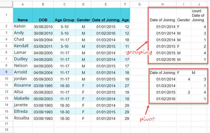
The following QUERY formula groups data by Date of Joining and Gender, then returns the count:
=QUERY(Sheet1!A1:F16, "SELECT E, D, COUNT(E) GROUP BY E, D", 1)
The result contains three columns:
- Date of Joining
- Gender
- Count of Date of Joining
This output is useful, but it’s still in a flat, row-based format.
Example 2: GROUP BY with PIVOT
Now, let’s use the PIVOT clause:
=QUERY(Sheet1!A1:F16, "SELECT E, COUNT(E) GROUP BY E PIVOT D", 1)
In this formula:
- Column D (Gender) is removed from the SELECT and GROUP BY clauses
- Instead, it is used in the PIVOT clause
As a result:
- The first column remains Date of Joining (column E)
- Additional columns are created for each distinct value in Gender
- Since Gender has two values (“M” and “F”), two pivoted columns appear
- The aggregated counts are displayed under these pivoted columns
This transforms row-based data into a cross-tabulated (pivot) layout.
Why Use PIVOT?
Pivoted QUERY results are especially useful for:
- Creating bar, column, line, or pie charts
- Building quick summary reports
- Preparing clean datasets for data visualization in Google Sheets
Can You Use PIVOT Without GROUP BY?
Yes—you can.
Here’s an example:
=QUERY(Sheet1!A1:F16, "SELECT COUNT(A) PIVOT E", 1)
In this case:
- The pivoted column (E – Date of Joining) creates one column per distinct date
- The count is calculated across the entire dataset
Try this formula yourself to see how QUERY behaves without an explicit GROUP BY clause.
Learn More About QUERY PIVOT
For advanced pivoting and reporting techniques, see this hub guide: QUERY Pivot & Reporting in Google Sheets
Sort QUERY Results Using ORDER BY Clause
The ORDER BY clause allows you to sort QUERY results based on the values in one or more columns in Google Sheets.
You can control:
- Which column(s) to sort by
- Sort direction (
ASCorDESC) - Sorting priority when using multiple columns
Example 1: Sorting by Column Identifiers
The following formula sorts the output by Name (column A) in ascending order:
=QUERY(Sheet1!A1:F16, "SELECT A, B, F ORDER BY A ASC", 1)
This formula sorts:
- Date of Birth (column B) in descending order, then
- Name (column A) in ascending order
=QUERY(Sheet1!A1:F16, "SELECT A, B, F ORDER BY B DESC, A ASC", 1)
When multiple columns are used in ORDER BY, sorting is applied from left to right.
Example 2: Sorting by Aggregated Results
You can also sort QUERY results using the output of an aggregation function.
=QUERY(Sheet1!A1:F, "SELECT F, COUNT(F) WHERE F IS NOT NULL GROUP BY F ORDER BY COUNT(F) DESC", 1)
This formula:
- Groups data by Age (column F)
- Counts the occurrences
- Sorts the result by the count in descending order
What Can Be Used in ORDER BY?
In the ORDER BY clause, you can sort by:
- Column identifiers (e.g.,
A,B,F) - Computed values, such as:
- Aggregation functions (
COUNT(),SUM(),AVG()) - Scalar functions
- Arithmetic expressions
- Aggregation functions (
Limit and Offset Rows in QUERY Function (LIMIT & OFFSET)
The purpose of the LIMIT clause (keyword) in the Google Sheets QUERY function is to restrict the number of rows returned by a query.
In the formula below, LIMIT 3 constrains the output to three rows, excluding the header row.
Example (LIMIT):
=QUERY(Sheet1!A1:F, "SELECT F, COUNT(F) WHERE F IS NOT NULL GROUP BY F ORDER BY COUNT(F) DESC LIMIT 3", 1)
The purpose of the OFFSET clause (keyword) is to skip a specified number of rows from the beginning of the result set.
Example #1 (OFFSET only):
=QUERY(Sheet1!A1:F, "SELECT * OFFSET 3", 1)
This formula skips the first three rows and returns the remaining rows.
Example #2 (LIMIT + OFFSET):
=QUERY(Sheet1!A1:F, "SELECT F, COUNT(F) WHERE F IS NOT NULL GROUP BY F ORDER BY COUNT(F) DESC LIMIT 3 OFFSET 1", 1)
In this example:
- The query first offsets (skips) one row
- Then applies LIMIT 3 to the remaining result set
So, OFFSET is evaluated before LIMIT in the QUERY function.
For practical use cases such as Top-N results, skipping ranked rows, and row-limiting strategies, see the hub: Top N and Row Limiting Techniques in Google Sheets QUERY.
Label and Format QUERY Output (LABEL & FORMAT Clauses)
Sometimes, a QUERY formula may return unfriendly or “ugly” column headers—especially when using expressions, scalar functions, or arithmetic operations.
For example, the formula below produces an auto-generated header such asdifference(year(Date of Joining), year(DOB)):
=QUERY(Sheet1!A1:F16, "SELECT A, YEAR(E) - YEAR(B)", 1)
As a result, the output may look like this:
Name | difference(year(Date of Joining), year(DOB))
Kelvin | 5
Andy   | 5
Chad   | 11
...
Let’s rename this header to something more readable.
Renaming Labels in the Header (LABEL Clause)
The LABEL clause allows you to define custom headers for one or more columns in the QUERY output.
Example:
=QUERY(Sheet1!A1:F16, "SELECT A, YEAR(E)-YEAR(B) LABEL YEAR(E)-YEAR(B) 'Age at the Time of Joining'", 1)
This formula replaces the default labeldifference(year(Date of Joining), year(DOB))
with the more readable header Age at the Time of Joining.
Related: Understand the LABEL Clause in Google Sheets QUERY.
Formatting Values in QUERY Output (FORMAT Clause)
The FORMAT clause is used to format dates, times, and numbers in QUERY results, similar to applying a Custom Number Format in Google Sheets.
Example:
=QUERY(Sheet1!A1:F16, "SELECT * FORMAT B 'YYYY-MM-DD'", 1)
This formats the date values in column B using the specified date pattern.
Related: Formatting Date, Time, and Numbers in Google Sheets QUERY.
Common QUERY Function Mistakes and Fixes
When using the Google Sheets QUERY function, you may encounter a few common issues. Most of these errors are easy to fix once you understand how QUERY interprets data.
1. Incorrect Header Argument (0 vs 1)
One of the most frequent mistakes is specifying the wrong header value in the QUERY function.
- Use
1if the data range includes a header row. - Use
0if the data range does not include headers.
Using the wrong header value can cause incorrect results or unexpected column references.
2. Incorrect Clause Order
The QUERY function requires clauses to follow a specific order. If the order is incorrect, the formula will return an error.
Always follow the correct clause sequence, such as:
SELECT → WHERE → GROUP BY → PIVOT → ORDER BY → LIMIT → OFFSET → LABEL → FORMAT
3. Using Incorrect Literals
Another common issue is not using the correct literals in QUERY statements.
Examples:
- Text values must be enclosed in single quotes (
'Text') - Dates must use the proper
DATE 'YYYY-MM-DD'format - Numbers should not be enclosed in quotes
Incorrect literal usage often results in errors or incorrect filtering.
These issues and their solutions have already been explained in detail in the sections above.
Conclusion: When and Why to Use Google Sheets QUERY Function
This guide has comprehensively covered everything you need to understand and confidently use the QUERY function in Google Sheets—from selecting and filtering data to grouping, pivoting, sorting, limiting results, and formatting output.
The QUERY function is especially powerful when you need:
- SQL-like data analysis without helper columns
- Dynamic reports and dashboards
- Clean, scalable formulas for large datasets
If you have any questions, edge cases, or use-case scenarios, feel free to drop them in the comments below.
Reference: Query Language Reference (Version 0.7)
Thanks for your time—happy querying!
Hi Prashanth,
I have a Google Sheets file (SPREADSHEET 02) where I am using a simple QUERY + IMPORTRANGE function to import data from another Google Sheets (SPREADSHEET 01).
=QUERY(IMPORTRANGE("SPREADSHEET 01 URL","Sheet1!A1:E"),"SELECT * WHERE Col4='✓'")Let’s say I am doing a check to each result in a new column (column 5) in SPREADSHEET 02 by adding the text “DONE”.
Now, if the row 2 in SPREADSHEET 01 turns the “X” to “✓”, it will ruin my checking progress.
My question is: Is there a function that can fix this issue?
Hi Bilal,
You need unique IDs in both sheets to link the records in both sheets. Other than the QUERY and IMPORTRANGE functions, you may also need to use the VLOOKUP or XLOOKUP functions to align the data. Please check this guide for an example.
Example: Align Imported Data with Manually Entered Data in Google Sheets.
I hope this is helpful!
Hello, is there is way to select a specific row, like “Select Row 2”?
Hi, Nick,
It’s possible! For example, I want to extract values in row # 5.
Range (Data): D1:E (D1:E1 contains field labels).
Solution # 1: Using Offset and Limit caluses.
=query(D1:E,"Select D,E limit 1 offset 3 ",1)or
=query({D1:E},"Select Col1,Col2 limit 1 offset 3 ",1)The formula offsets three rows + header row. So you will get the fifth row.
Solution # 2: By adding row number column.
=ArrayFormula(query({row(D1:D),D1:E},"Select Col2,Col3 where Col1=5",1))I have a query that I’m trying to eliminate returning 0s, but because they’re not quite 0 (infinite number).
I can’t seem to filter them out of my query correctly. Is there a way to get around this?
Hi, Richard Corneau,
Your shared sheet is in COMMENT mode. So commented the formula there.
How can we sort a column in descending order in the query function for % values? 100 % is not getting at the top.
=QUERY('Negative_Report - Data'!A6:M141,"Select A,H Order by H DESC LIMIT 20")H is the percentage column.
Hi, Daniel Malakar,
Your formula seems correct. Please check the values in column H for formatting. It might be text formatted.
Hello Prashanth,
May I ask you to help me with this formula?
I’ve copied it from another GS spreadsheet and thought that is working well, but recently found that this formula is using similar results to make a “decision” of what to select. I’m almost sure that it’s because of Wildcard symbols.
I was googling something like “google sheets query formula equals to comparison operator” but haven’t found anything useful.
Here is the formula:
=IF(ISTEXT(O3),QUERY('Sheet2'!$A$2:'Sheet2'!$X$200, "select C where A like '%" & O3 &"%' limit 1",""))It is selecting from C, but if in A column it finds “02.03.00.124” firstly and “02.03.00.12” after, so the result of C would be from first A (02.03.00.124).
I just need something like “select C where A equals to “O3”, but it doesn’t work, obviously 🙂
Hi, Vladislav,
Use “Contains” substring match as below.
=QUERY(Sheet2!A2:X200, "select C where A contains '03'",0)I have 2 Columns.
“SEO 12”
“SEO, Retails 12,34”
“E-commerce 56”
I need to return values from Column A containing 12. I need to get “SEO” and “SEO, Retails”.
How do I do it?
Hi, Abhidith Shetty N,
Use the CONTAINS clause.
=query(A1:B,"Select * where A contains '12'")You can find related tutorials (CONTAINS, MATCHES, and LIKE complex comparison operators) on this blog.
The FILTER function will also work.
=filter(A1:B,regexmatch(A1:A,"12"))Hello there. Nice tutorial.
I am attempting a query without multiple where clauses. This works as I expect.
=QUERY(TravelPlus!A2:U110,"SELECT G WHERE ((lower(A) = 'john smith')) AND ((lower(B) = 'july 26 - august 25')) limit 1", false)Then, I’d like to replace the second clause ‘july 26 – august 25’ with a cell reference. Based on searching around, I think it should be this, but I receive a formula parse error.
=QUERY(TravelPlus!A2:U110,"SELECT G WHERE ((lower(A) = 'john smith')) AND ((lower(B) = "'&A1&'")) limit 1", false)Any idea what I might be doing wrong?
Hi, Chris C,
You were very close!
Here is the correct Query formula.
=QUERY(TravelPlus!A2:U110,"SELECT G WHERE lower(A) = 'john smith' AND lower(B) = '"&A1&"' limit 1", false)Search the term “literals” (using Ctrl+F [browser search not my blog search]) within this Query function tutorial and you can find a related link.
Can you combine a WHERE clause with a MATCH? For example, I want the column being evaluated to be a variable in a dropdown. I’ve tried this and it returns a #N/A (empty result).
=query({$C$2:$F},"Select Col1 where 'Col"& match($A$2,$C$2:$F$2,0)&"' ''",1)If I highlight just the match function, it gives me a correct result (1, 2 or 3) and if I swap the match out with, say, Col2, the query works fine.
Does match not work in a where clause of is my syntax wrong?
Hi, Chris Rosendin,
Here is the correct usage of the Match spreadsheet function within the Query Where clause.
=query({$C$2:$F},"Select Col1 where Col"&match($A$2,$C$2:$F$2,0)&"<> ''",1)Hi!! my Query function returns an “N/A”. How can I remove that?
Wrap the formula within IFNA like;
=IFNA(Query())I’m having an issue when I use this function with IMPORTRANGE. It doesn’t copy over any cells if they have special characters, for example, Zipcodes or phone numbers with
( )or-Those cells do come over fine if I just do IMPORTRANGE so I am wondering what the workaround is to still get that when using Query to only pull data over
"where Upper (col4)='X'"Thanks.
Hi, Chanel,
If you have permission to edit the source file;
Format the column that contains the Zipcodes, special characters, etc. to text (Format > Number > Plain text).
Then use the Query as per the below example.
=query(importrange("URL","Sheet1!A1:E10"),"Select * where upper(Col5)='X'")Please use
Col5, notcol5.If don’t, use the To_text function within your Query ‘data’
Example:
I am importing the column range A1:E10 if column E contains “X”. In this, column D contains special characters.
=ArrayFormula(query(to_text(importrange("URL","Sheet1!A1:E10")),"Select * where upper(Col5)='X'",1))This has one drawback. It will convert all the outputs to text format.
Do you know of a workaround for the missing SQL IN condition in the Google Sheets Query Function, e.g.
"SELECT * FROM tbl_country WHERE country_code IN ('UK', 'DE','AT')"?Hi, Andi,
Please see the String Comparison operators especially the ‘Matches’. The links provided within this tutorial.
If you want me to write a formula that specific to your problem, let me view the sample (no personal/sensitive data) of your Sheet.
Best,
See this new article – The Alternative to SQL IN Operator in Google Sheets Query (Also Not IN).
I have a question. I’d love help. Long story short, I have a sheet that shows lists of students and the bus that they ride on for our school.
Example: Teacher A’s Class
Column A: Student
Column B: Bus Number
On a separate sheet, I want to create a query so that only the students on Bus 1 show up on that sheet. Then another sheet where only students on Bus 2 show up. I am struggling to figure it out. Any help or recommendations for how to learn this would be awesome!
Hi, Rachel,
I assume the list of students is in Sheet1 (tab name) and the first row in that contains the column names (field labels).
Here is the Query to filter the Students on Bus 1. Enter this Query in Sheet2.
=query(Sheet1!A1:B,"Select A where B=1",1)If the bus numbers are text strings like Bus 1, Bus 2 then use the below Query.
=query(Sheet1!A1:B,"Select A where B='Bus 1'",1)You can change
B=1toB=2orB='Bus 1'toB='Bus 2'to filter the students on Bus 2.Best,
Hi, I am working on a translation glossary of terms for myself for my job and was hoping to use the Query function to separate and show the term you’re looking for by typing it in.
Unfortunately, I find this guide to be pretty vague and the descriptions of how to use each function/equation quite lacking. Am I just not using the right function, or am I using this function incorrectly?
query(DataList!C1:D1,"select A,B,C,D where C='"&E3:E1000&"'")C1:D1 is where I want my search box, E3:E1000 are the cells in which I have the tags (denoted by # much like on Instagram) pertaining to each vocabulary term. C3:D1000 would be the locations for the terms in each language.
Thank you.
Michelle
Hi, Michelle V.,
This part of the Query Where clause is wrong.
where C='"&E3:E1000&"'You can only specify one cell (one criterion) this way like;
where C='"&E3&"'If you want to use several criteria, then you may use the Matches regular expression match in Query.
To give you a correct formula, I may want to see your Sheet. If your Sheet contains personal data, instead share a demo Sheet with some mockup data.
Best,
I’m trying to combine data from multiple tabs to create a master product database. There is a chance we will add new products in the future and I want to know if there is a way to get the “data” section of the Query Function to automatically expand with the new tab names, rather than adding the tab names into the master query equation. I’m open to creating a database of tab names, but thus far have not had success getting the data section to recognize text within a cell as an address.
Hi, Jessica,
Here is one workaround – How to Include Future Sheets in Formulas in Sheets.
I’m trying to query multiple fields but having an issue. i.e,
=QUERY(Sheet1!A2:BQ,"select B,C,U,W where AC='Yes'")and
=QUERY(Sheet1!A2:BQ,"select B,C,AE,AG where AM ='Yes'")So if AC is true I need 5 fields, if AM is true I need the same 2 fields and 3 different fields, etc. (there are 5 in total). And I’d like to them order by B desc. I can do multiple separate query’s but not all together. I thought I could use an or but it’s not working.
Hi, Mustom,
It was time taking still I have managed create an example Sheet based on your formula. Your formulas seem working independently. But I could not find the logic. I am unsure whether the same row in AC and AM contains “Yes”.
I may be able to help if you leave an example sheet and in that the output that you are expecting.
Best,
Try to finish the query by ;0 like,
=query(DataList!A1:F16, "select A,B,F";0)Is it working?
Hi, Nico,
I understand you are talking about Query Headers. It’s optional and useful when your data has headers in multiple rows. Also, there is a tricky way of using it to combine columns – The Flexible Array Formula to Join Columns in Google Sheets.
Now regarding your question, my answer is “it does work”. But you may use a comma instead of semicolon but that depends on your locale setting (File menu > Spreadsheet setting).
Without seeing what you are trying to achieve and your locale, I can’t comment further.
Thanks.
How to remove the broken line in the fields retrieved by the QUERY function?
Please explain little more 🙂