


The ISLOGICAL function in Google Sheets is an info type function. That means you can use it to gather information about
The ISLOGICAL function is useful to identify the Boolean values that denoted by TRUE or FALSE in Google Spreadsheets.
A cell may contain either of the above Boolean values in three ways – as an output of Logical test, by inserting tick boxes, or by manually entering.
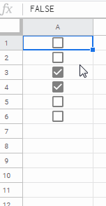
Tick Boxes in Google Sheets Placing the Boolean Values in Cells
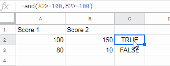
The Logical Formula That Returns the Boolean Values in Cells
Here is one example with the Logical AND function which returns the TRUE or FALSE values.
There are other logical functions like IF, OR, XOR etc. that can return similar values. You can find that functions under the heading “Logical” in my Functions Guide.
Just TRUEFALSE
Purpose:
The one and only purpose of the function ISLOGICAL in Google Docs Sheets is to check whether a value is TRUE or FALSE.
Example to the Use of the ISLOGICAL Function in Google Sheets
In the below examples, the ISLOGICAL formula tests the values in the column C.
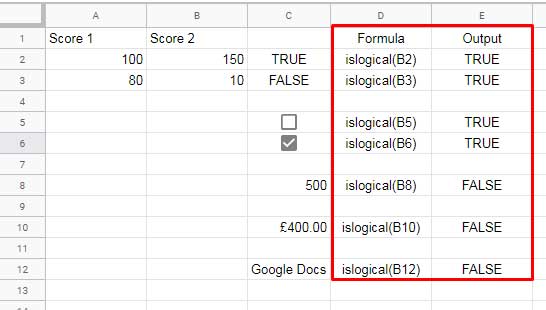
The interesting fact is that the ISLOGICAL function tests the presence of Boolean values and also returning the Boolean Values as the output.
To convert that output to numerical 1 or 0, change the formula as below.
The formula in cell E2:
=--islogical(C2)The Use of ISLOGICAL Function in an Array in Google Sheets
This info type function can be useful to test a set of values using ArrayFormula. If you want to get the info of the values in C2:C12, you can use the formula as below.
=ArrayFormula(islogical(C2:C12))Practical Use of Google Sheets ISLOGICAL Function
Just learning an info type function is not enough. You must know where you can make use it in your data manipulation.
I am going to use this function in two entirely different scenarios.
- As a worksheet formula.
- As a custom formula rule in conditional formatting.
Example to the Use of ISLOGICAL with FILTER Function
Problem: Filter only those rows that contain a tick box in column B.
=filter(A2:B13,ISLOGICAL(B2:B13))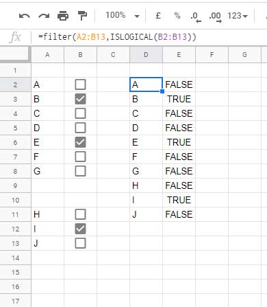
Highlight Boolean Values Using ISLOGICAL in Google Sheets
To avoid screenshot I am going to use the sample data used in the above example. But this time includes not only column A and B but also the columns D and E.
Steps:
- Select the range A1
:E13 . - From the menu Format, select “Conditional formatting”
- Select “Format rules” as “Custom formula is”
- Enter the following ISLOGICAL formula in the provided field.
=islogical(A1)This will conditional format all the cells that contain TRUEFALSE
Additional Reading: