")
")


")


")

")
")
 in Excel & Google Sheets")


To insert check marks and cross marks, we can use characters, while for tick boxes, we can use data validation in Google Sheets.
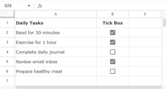
We can use check marks and tick boxes to mark completed tasks, verified records, etc.
While tick boxes are interactive, check marks are not; they are simple characters. To use the latter effectively in your data, you might want to apply logical tests.
How to Insert Tick Boxes in Google Sheets
Currently, you can insert tick boxes in a selected range in three ways: via the Insert menu, data validation, or by choosing the column type in a table.
The tick box value when ticked is TRUE and unticked is FALSE, regardless of the option that you choose to insert it. Furthermore, if you insert the tick boxes via the Insert menu or the table column type feature, you can customize them using data validation.
Option 1: Via Insert Menu
The easiest method to insert a tick box is using the Insert menu. If you want it in cell B2, navigate to cell B2 and click on the Insert menu, then select Tick Box. If you want it in a cell range, select the cell range and follow the same steps.
Option 2: Via Data Validation
Another option is through data validation. Knowing how to insert tick boxes via data validation is essential as it offers some customization.
To do this, navigate to the cell or select the cell range where you want to insert the tick boxes.
- Click on Data > Data validation.
- Within the Data Validation rule sidebar panel, click Add Rule.
- Under “Criteria”, select Tick Box.
Additional Data Validation Settings for Tick Boxes:
The default values in the tick boxes are TRUE (ticked) and FALSE (unticked). You can customize this by clicking the “Use custom values” checkbox within the sidebar panel.
For example, you can replace TRUE with 1 (ticked value) and FALSE with 0 (unticked value). This can help you when you face issues using the default TRUE or FALSE values in formulas due to language settings.
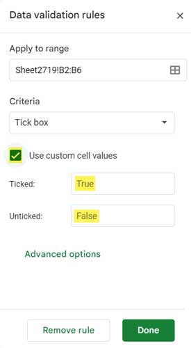
If you click “Advanced options,” you will see options to set warnings when somebody overwrites the tick boxes with other values. This is similar to other data validation rules.
Option 3: Via Table Column Type
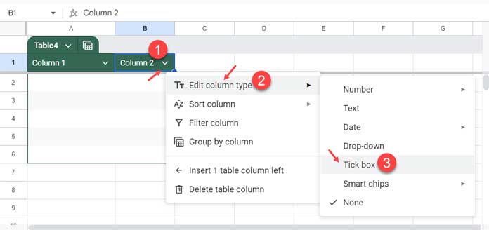
Let me explain this step-by-step by creating an empty table in Google Sheets.
- In an empty sheet, select A1:B6.
- Click Format > Convert to Table. This will insert a blank table. Assume you want the tick boxes in column B.
- Click the drop-down in column 2 and select Edit column type > Tick box. This will insert tick boxes in the range B2:B6.
Activating the Inserted Tick Boxes
You can activate the tick boxes in two ways: by clicking the tick box or by tapping the space bar.
How to Insert Check Marks in Google Sheets
Check marks are characters. You can add them to the required cell in two ways.
By entering the following formulas:
- To insert a check mark in a cell:
=CHAR(10004) - To insert a cross mark in a cell:
=CHAR(10006)
Or you can copy-paste from here:
- Check Mark: ✔
- Cross Mark: ✖
Example of Using Check Marks and Cross Marks in Logical Tests
Since check marks and cross marks are not interactive, the best way to use them is in logical tests.
In the example below, we have a few student names in column A and their marks in column B.
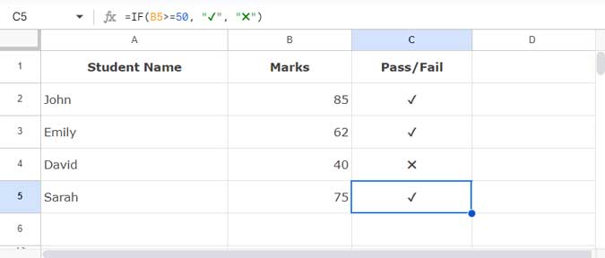
In cell C2, we can use the following formula to return a check mark if the student has scored greater than or equal to 50, or a cross mark:
=IF(B2>=50, "✔", "✖")Then drag the formula down.
Resources
- Assign Values to Tick Box and Total It in Google Sheets
- Change the Tick Box Color While Toggling in Google Sheets
- 10 Best Tick Box Tips and Tricks in Google Sheets
- Check-Uncheck a Tick Box based on the Value of Another Cell in Google Sheets
- How to Convert TRUE or FALSE to Check Boxes in Google Sheets
- Tick Mark: Lock and Unlock Cells Using Checkboxes in Google Sheets
- Vlookup in Checkbox Checked Rows in Google Sheets
- Highlighting Multiple Groups and Control Tick Boxes in Google Sheets
- Create a List from Multiple Column Checked Tick Boxes in Google Sheets