Similar to columns, which is widely popular, we can use infinite row reference horizontally in Google Sheets. I find it very useful in a few instances
Entire column and entire row may be sometimes quite confusing for Google Sheets users. That’s why I have included the word “Horizontally” in the title.
The entire column here means entire cells in a column. That entire cells are actually different rows.
The entire row here means entire cells in a row. In that, each cell is in different columns.
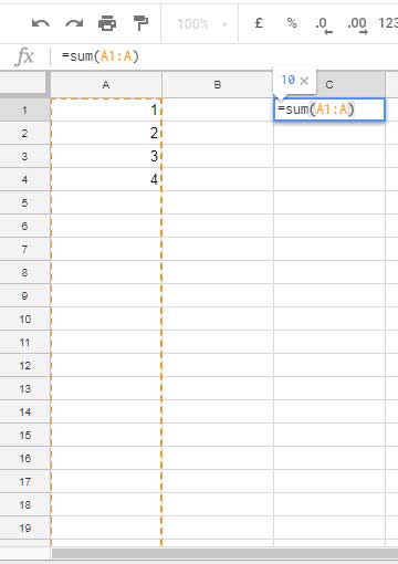
A1, A2, A3 … is an example to an entire column. In formulas, you can refer entire columns as below.

In Google Sheets how to use infinite row reference in formulas?
Infinite Row Reference in Google Sheets Formulas
To include infinite row reference in formula use the reference as below.

To include multiple rows in infinite row reference you can follow the below method. Here the formula covers the first five rows infinitely.
=A1:5What’s the Benefit of Using Infinite Row Reference in Google Sheets
When you import an entire spreadsheet using Importrange, use infinite row reference. This can ensure that the imported table accommodates future changes in the source table like the
Infinite Rows in Importrange:
In my source data, in Sheet1, I have maximum columns in the Sheet is 26 (A to Z) and rows are 1000. In that, I have data in the range A1
You can import the range A1:T7 as below.
=importrange("Enter your source file URL","Sheet1!A1:T7")Change the reference to “Sheet1!A1:1000” so that you can ensure that all the new columns in the source are getting imported.
Warning: This can slowdown the performance of your Spreadsheet.
Infinite Row Reference in Hlookup:
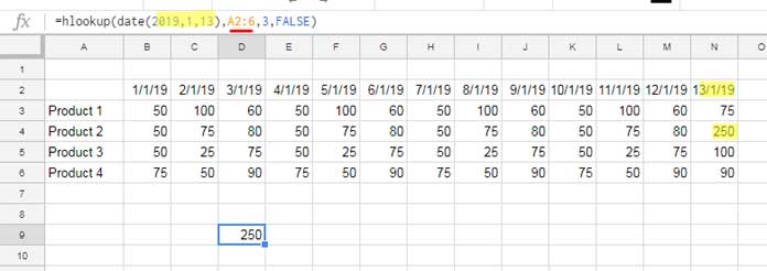
Another example is with Hlookup. If you have a growing number of columns like one column each for each date, then use the Hlookup as below.

Infinite Row Ranges in Expanding Formula:
Before winding up this tutorial, here is one more example.
It’s common to use Isblank or IF+Len combo to control expanding formulas in columns. Can we use any of these formulas in infinite rows?
Yes. Here is that example.
The below formula populates the sequential numbers in an entire row but up to the column that contains values in the second row.
=ArrayFormula(if(len(A2:2),column(A2:2),))
Conclusion
In addition to the above formula examples, you can find Infinite Row Reference useful in functions like Query, Index, Match etc.
That’s all for now! Hope you have enjoyed the stay.
Related Reading:


Thank you so much. It helped me a lot 🙂
Hi Prashanth,
It’s not working, please refer to the sheet and kindly do help.
Hi, Hima,
Added the formula on your Sheet.
Your sum range starts from column A in the ‘Days’ tab and you are trying to insert the formula (get the offset sum) in column B in a different tab.
Since both the columns are different you must have modified the formula as per the details under the ‘Usage Note 1’ on this post.
How to Sum Every N Cells to the Right or Bottom in Google Sheets
I know I didn’t share this post earlier.
Best,
Hi,
I have the days in columns in one sheet and another sheet I have to select the Monday to Friday cell range manually, is there any formula to drag horizontally so that can auto-update the cell reference range or number
If I drag horizontally am getting the
=SUM(Raw!IN2:IQ2)=SUM(Raw!IO2:IR2) instead I need to get next five cells means from IR2:IV2=SUM(Raw!IP2:IS2) instead I need to get next five cells means from IW2:IZ2Example :
=sum(Raw!B2:D2)(adding five working days date range)=sum(Raw!E2:I2)=sum(Raw!J2:M2)For me, that is possible with a helper row.
For example, my values are in B2:2.
In B3 I will use this array formula and then hide the row.
=ArrayFormula(if(len(B2:2),sequence(1,columns(B2:2),0,4),))The below formula is for cell B4. Drag to the right to sum after offsetting 5 columns each.
=sum(offset(B2:2,0,B3,1,5))If you want any additional info, please let me know. I’ll try to explain it by writing a post.
Best,
The same without the helper row!
=sum(offset($B$2,0,(column()-column($B$2))*5,1,5))This formula is for cell B3. Darg to the right.