How to Import Every Nth Row in Google Sheets

If you’re working with large datasets, you may want to extract just every few rows—say, every third row—to simplify analysis or visualization. This tutorial explains how to import every nth row in Google Sheets, using clean, formula-based methods that work across sheets in the same file or even between different Google Sheets files.

Table of Contents

What Do We Mean by “Import”?

Before we dive into the how, let’s clarify what we mean by import in this context.

In Google Sheets, importing data doesn’t always mean pulling it from an entirely different file. It could be from:

Another tab (sheet) within the same file
An external Google Sheets file using IMPORTRANGE

The good news is, the formula to import every nth row in Google Sheets remains the same. The only part that changes is whether your data comes from a local tab or an external spreadsheet.

Decide Where to Start: First Row or Nth Row?

One flexible aspect of the method we’re using is that you can choose to:

Start from the first row of your dataset
Or start from the nth row itself (e.g., start from the 3rd row and then pick every 3rd row from there)

We’ll share both formulas below so you can use the one that fits your need.

Formulas to Import Every Nth Row in Google Sheets

Formula 1: Start from the First Row

=LET(data, Sheet1!A2:C, n, 3, CHOOSEROWS(data, SEQUENCE(ROUNDUP(ROWS(data)/n), 1, 1, n)))

Formula 2: Start from the Nth Row

=LET(data, Sheet1!A2:C, n, 3, CHOOSEROWS(data, SEQUENCE(ROUNDUP(ROWS(data)/n), 1, n, n)))

In both formulas:

data is your input range — for example, Sheet1!A2:C (for same-sheet data) or IMPORTRANGE("...", "Sheet1!A2:C") (for external data)
n is the interval—for example, 3 for every third row

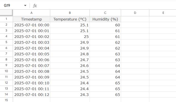
Example Dataset

Here’s a sample dataset in range A1:C (from a tab named Sheet1):

Let’s now explore how to import every 3rd row from this data.

How to Import Every Nth Row from an External Google Sheet

If your data is in a different Google Sheets file, use IMPORTRANGE to bring it into your current sheet. Here’s how:

In cell A1 (or any blank cell), enter:

=IMPORTRANGE("https://docs.google.com/spreadsheets/d/your-spreadsheet-id/edit", "Sheet1!A2:C")

Note: We used A2:C instead of A1:C to skip the header row.

The formula may return a #REF! error at first—hover over the cell and click “Allow Access”.
Now that the data is imported, apply the earlier formula to import every nth row from that imported range by replacing the data in that formula with this IMPORTRANGE formula:

Every 3rd Row, Starting from the First Row:

=LET(data, IMPORTRANGE("https://docs.google.com/spreadsheets/d/your-spreadsheet-id/edit", "Sheet1!A2:C"), n, 3, CHOOSEROWS(data, SEQUENCE(ROUNDUP(ROWS(data)/n), 1, 1, n)))

Timestamp	Temperature (°C)	Humidity (%)
01/07/2025 00:02:00	25	61
01/07/2025 00:05:00	24.8	63
01/07/2025 00:08:00	24.5	64
01/07/2025 00:11:00	24.4	65

Every 3rd Row, Starting from the 3rd Row:

=LET(data, IMPORTRANGE("https://docs.google.com/spreadsheets/d/your-spreadsheet-id/edit", "Sheet1!A2:C"), n, 3, CHOOSEROWS(data, SEQUENCE(ROUNDUP(ROWS(data)/n), 1, n, n)))

Timestamp	Temperature (°C)	Humidity (%)
2025-07-01 00:02	25	61
2025-07-01 00:05	24.8	63
2025-07-01 00:08	24.5	64
2025-07-01 00:11	24.4	65

Replace the sample URL with the actual URL of your source file.

Import from Another Tab in the Same File

This is even simpler. You just refer to the range in the same file directly—no IMPORTRANGE needed.

Every 3rd Row, Starting from the First Row:

=LET(data, Sheet1!A2:C, n, 3, CHOOSEROWS(data, SEQUENCE(ROUNDUP(ROWS(data)/n), 1, 1, n)))

Every 3rd Row, Starting from the 3rd Row:

=LET(data, Sheet1!A2:C, n, 3, CHOOSEROWS(data, SEQUENCE(ROUNDUP(ROWS(data)/n), 1, n, n)))

Formula Explanation

Here’s a breakdown of what’s happening:

LET(...) is used to define the data range and the interval n
SEQUENCE(ROUNDUP(ROWS(data)/n), 1, start, n) generates the row positions to extract
CHOOSEROWS(data, ...) selects only those rows from the dataset

For example, if your data has 13 rows and n = 3, the SEQUENCE will produce:

{1; 4; 7; 10; 13}  // if starting from row 1

{3; 6; 9; 12}  // if starting from row 3

This is a clean, no-script approach to importing every nth row in Google Sheets.