In Google Sheets, you can insert in-cell images primarily in two ways: using the IMAGE function or by navigating to Insert > Image > Insert an Image in the Cell. Both methods allow you to display images within cells, and these images can be used in lookup functions like VLOOKUP.

The Insert > Image option lets you add images from various sources, such as your computer, Google Drive, or by providing a URL. However, the IMAGE function requires a URL specifically.

The advantage of the function is that it gives you control over the display size and aspect ratio of the image within the cell, which isn’t possible through the Insert menu. Here’s a detailed tutorial on using the IMAGE function in Google Sheets.

IMAGE Function Syntax

Syntax:

IMAGE(url, [mode], [height], [width])

There are four arguments in the IMAGE function. Let’s go over them with examples.

Arguments and Examples:

URL

This is the URL of the image you want to display in the cell.

Example: To display an image from a URL, such as this one:

=IMAGE("https://infoinspired.com/wp-content/uploads/2024/04/iso-logo-ii-4.png")

Alternatively, if you place the URL in cell A1, you can use:

=IMAGE(A1)

Note: Make sure the URL is not enclosed in double quotes if it’s referenced in a cell.

MODE

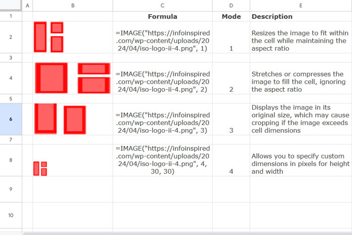
The mode argument controls how the image is resized within the cell. Here are the options:

• 1 (default): Resizes the image to fit within the cell while maintaining the aspect ratio. This is often the best option for a clear display.
  =IMAGE("https://infoinspired.com/wp-content/uploads/2024/04/iso-logo-ii-4.png", 1)
• 2: Stretches or compresses the image to fill the cell, ignoring the aspect ratio.
  =IMAGE("https://infoinspired.com/wp-content/uploads/2024/04/iso-logo-ii-4.png", 2)
• 3: Displays the image in its original size, which may cause cropping if the image exceeds cell dimensions. To view the entire image, adjust the cell size accordingly.
  =IMAGE("https://infoinspired.com/wp-content/uploads/2024/04/iso-logo-ii-4.png", 3)
• 4: Allows you to specify custom dimensions in pixels for height and width, which can be useful when resizing images to specific sizes.
  =IMAGE("https://infoinspired.com/wp-content/uploads/2024/04/iso-logo-ii-4.png", 4, 25, 25)
  • Height
    (Only for mode 4) Sets the image height in pixels.
  • Width
    (Only for mode 4) Sets the image width in pixels.

Using the IMAGE Function with Dynamic Arrays

If you have a series of images stored in the same folder with sequential naming (e.g., iso-logo-ii-1.png, iso-logo-ii-2.png, etc.), you can use the IMAGE and SEQUENCE functions together to load all images in their own cells dynamically.

Example:

=ARRAYFORMULA(IMAGE("https://infoinspired.com/wp-content/uploads/2024/04/iso-logo-ii-" & SEQUENCE(4) & ".png"))

Note: You cannot use volatile functions (e.g., NOW, RAND, RANDARRAY, COINFLIP) in the base URL for the IMAGE function, as they cause the URL to update constantly, which the IMAGE function does not support.

Using the IMAGE Function with Lookup Functions

The IMAGE function enables in-cell images to be used with lookup functions like VLOOKUP, XLOOKUP, LOOKUP, and HLOOKUP. This can help display images based on a lookup value.

Example: If cell A1 contains the text “logo” and cell B1 contains an IMAGE formula, you can use:

=VLOOKUP("logo", A1:B1, 2, FALSE)

Or with XLOOKUP:

=XLOOKUP("logo", A1, B1)

This technique is useful for displaying images such as meal photos based on the selected meal in a restaurant menu, country flags by country names in a list, and more.

Resources

• How to Copy and Paste Images from Excel to Google Sheets
• Insert Images in Cells Without Formula in Google Sheets
• Copy Image From One Spreadsheet to Another in Google Sheets