Here, you can learn how to use the DSUM function in Google Sheets through a simple example, accompanied by supporting pictures.

As the name implies, the DSUM function allows you to obtain the sum of values in any numeric field within a database, based on specified criteria.

The DSUM function shares similarities with another Google Sheets function known as SUMIF/SUMIFS, and both can yield similar results.

However, in my opinion, SUMIF is more user-friendly. One notable distinction between DSUM and SUMIF/SUMIFS is that the former is a database function, returning the sum of values selected from a database table or similar array/range using an SQL-like query. In contrast, the latter is of a logical type.

For more in-depth information, you can refer to my tutorial on the Difference Between SUMIFS and DSUM in Google Sheets.

Now, let me provide further details on how to effectively use the DSUM function in Google Sheets.

How to Use the DSUM Function in Google Sheets

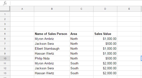
Similar to my other spreadsheet tutorials, it’s recommended to begin by creating a database table, as illustrated below, to practice and experiment with my DSUM formula.

Ensure that you maintain the data range reference B5:D13, as this will enable you to easily follow and adapt to my formula explanation.

If you prefer, you can duplicate (copy) my sample sheet by clicking the button below.

Sample Sheet

Now, let’s take a closer look at how the DSUM function works.

Google Sheets DSUM Function Syntax Explained (With Picture)

Syntax of the DSUM Function in Google Sheets:

DSUM(database, field, criteria)

Arguments:

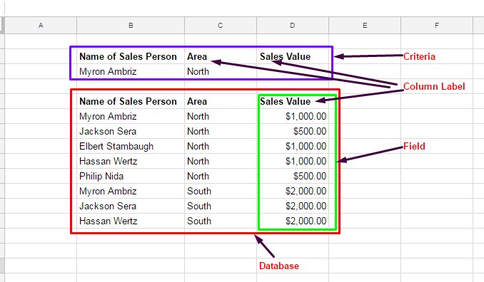
• database: This is the data range to consider. The first row should contain labels for each column’s values. In the example, the range B5:D13 is the “database,” with labels in the first row (B5:D5).
• field: Indicates which column in the database contains the values to be extracted and operated on. In the example, column 3 is used as the field, representing the numeric values. The formula will sum this column based on the given criteria.
  • You can use either the column number directly (e.g., 3) or the column name within double quotes (e.g., “Sales Value”).
• criteria: The range containing conditions or criteria for filtering the database values before operating. It should include at least one column name (field label) and one cell below it. You can copy-paste column names into another range for criteria and fill only the required ones.
  • In the example, the criteria are within the range B2:C3.

I understand it may seem a bit confusing, so I’ve provided a screenshot for clarification.

The specific use of the ‘criteria’ argument is detailed below.

Examples

Assuming you have prepared the sample ‘database’ in the range B5:D13 as mentioned earlier, the next step is to specify the criteria, as shown in the screenshot above.

To set the criteria:

1. Copy the labels “Name of Sales Person,” “Area,” and “Sales Value” from B5:D5.
2. Paste these labels into B2:D2.

Now, let’s say we want to total the Sales Value of the person “Myron Ambriz” in the “North” area using the DSUM in Google Sheets.

For testing, enter “Myron Ambriz” in cell B3 and “North” in cell C3. Your criteria should look like this:

Next, enter the DSUM formula in cell D3, considering multiple criteria:

=DSUM(B5:D13, 3, B2:C3)

In this formula, B5:D13 represents our database, 3 is the field (the column to sum), and B2:C3 is the criteria range.

Note: You can replace the field #3 (column number) with the cell reference D2, which contains the column name. This provides flexibility in using either the column number or the column name for the DSUM function.

If you insert this formula in cell D3, you should get the result as $1,000.

Now, let’s expand the criteria and observe the result:

Formula:

=DSUM(B5:D13, 3, B2:C4)

Result: $3,000.

This demonstrates how to use DSUM in both Google Sheets and Microsoft Excel.

Can I Use DSUM Criteria Inside the Formula in Google Sheets?

Yes, you can! However, the approach is different compared to how we handle SUMIF or SUMIFS criteria.

Take a look at the last formula criterion in the range B2:C4 above. It can be replaced with the following virtual array inside the formula:

{{"Name of Sales Person"; "Myron Ambriz"; "Myron Ambriz"}, {"Area";"North";"South"}}

This formula part creates a virtual array containing the criteria and column names (field labels). Curly Braces are used to create the array, and it has two parts: Vertical Array 1 and Vertical Array 2.

• Vertical Array 1: {"Name of Sales Person"; "Myron Ambriz"; "Myron Ambriz"}
• Vertical Array 2: {"Area"; "North"; "South"}

The outer Curly Braces and the comma separator stack these two vertical arrays horizontally.

The complete formula will be:

=DSUM(B5:D13, 3, {{"Name of Sales Person"; "Myron Ambriz"; "Myron Ambriz"}, {"Area"; "North"; "South"}})

For forming the virtual array, instead of Curly Braces, you can use the VSTACK and HSTACK functions. Then the criteria will be:

HSTACK(VSTACK("Name of Sales Person", "Myron Ambriz", "Myron Ambriz"), VSTACK("Area", "North", "South"))

For more in-depth information on using multiple conditions in the DSUM function, you can refer to the tutorial: AND, OR in Multiple Criteria DSUM in Google Sheets (Within Formula).

Date, Number, and Text Criteria in DSUM in Google Sheets

In our example, all the criteria are text strings because our sample database doesn’t have a date field.

I’ve prioritized providing a clear understanding of the DSUM function with minimal examples. You might need to use date, timestamp, and number criteria, along with comparison operators.

For detailed guidance on handling criteria in DSUM in Google Sheets, please refer to my tutorial: How to Properly Use Criteria in DSUM in Google Sheets.

Also, check out the additional resources below.

Resources

1. The Ultimate Guide to Using Criteria in Database Functions in Google Sheets.
2. How to Use Multiple Sum Columns in the DSUM Function.
3. How to Do a Case Sensitive DSUM in Google Sheets.
4. Exact Match of Criteria in Database Functions in Google Sheets.
5. How to Use Date Difference As Criteria in DSUM in Google Sheets.