You can return unique rows in Google Sheets QUERY with the help of the UNIQUE and SORTN functions. These powerful tools allow you to filter, summarize, and deduplicate your data effectively.

We commonly use the UNIQUE function to remove duplicate values. SORTN can achieve similar results but works differently, especially when using tie mode 2 to return the first instance of each group.

The purpose of combining Google Sheets QUERY with UNIQUE or SORTN is to apply these functions to filtered or aggregated (queried) data.

Syntax to Return Unique Rows in Google Sheets QUERY

• UNIQUE + QUERY Syntax:
  =UNIQUE(QUERY(...))
• SORTN + QUERY Syntax:
  =SORTN(QUERY(...), 9^9, 2, column_index_to_unique, 1)

Note: The actual QUERY statements are omitted above, as they vary depending on your dataset and filtering conditions. You’ll see full examples in the sections below.

Scenario 1: Return Unique Rows from a Filtered Column

Let’s say you have a two-column dataset with Items in column B and their Transaction Type in column C. We want to return unique items where the transaction type is “Purchase”.

Example Formula:

=QUERY(B2:C, "SELECT B WHERE C = 'Purchase'")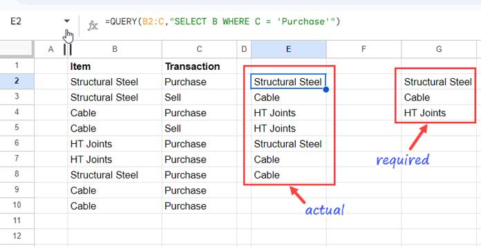

This filters the data to show only items with a “Purchase” transaction. To return unique rows in Google Sheets QUERY, wrap the formula with the UNIQUE function:

=UNIQUE(QUERY(B2:C, "SELECT B WHERE C = 'Purchase'"))

This setup removes duplicates and ensures you’re only seeing the unique purchased items. You can also use multiple conditions in your QUERY statement as needed.

Scenario 2: Return Unique Rows Based on the Most Recent or Oldest Dates

Now consider a dataset with three columns: Item (A), Transaction (B), and Date (C). We want to get a list of unique items purchased, along with either the most recent or oldest purchase date.

Example QUERY:

=QUERY(A2:C, "SELECT A, C WHERE B = 'Purchased'")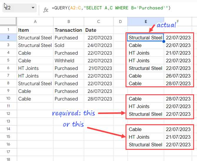

However, simply applying the UNIQUE function won’t give us the desired result because both the Item and Date values are returned—and dates vary. Instead, we need to determine either the most recent or oldest date per item.

Method 1: Return Unique Rows in Google Sheets QUERY Using SORTN

To get the most recent purchases, sort the data by item (ascending) and date (descending), then use SORTN to return the first row for each item:

=SORTN(QUERY(A2:C, "SELECT A, C WHERE B = 'Purchased' ORDER BY A ASC, C DESC"), 9^9, 2, 1, 1)

• 9^9 specifies a large number of rows to return.
• 2 is the tie mode to group by unique values.
• The final 1, 1 sets the unique-by column index (column A in this case).

To get the oldest purchases, sort by item and date in ascending order:

=SORTN(QUERY(A2:C, "SELECT A, C WHERE B = 'Purchased' ORDER BY A ASC, C ASC"), 9^9, 2, 1, 1)

This is a reliable way to return unique rows in Google Sheets QUERY when working with grouped data.

Method 2: Use QUERY Only (No Wrappers) to Return Unique Rows

You can also achieve similar results using just the QUERY function by aggregating the date values per item:

• Most recent purchase per item:
  =QUERY(A2:C, "SELECT A, MAX(C) WHERE B = 'Purchased' GROUP BY A LABEL MAX(C) ''")
• Oldest purchase per item:
  =QUERY(A2:C, "SELECT A, MIN(C) WHERE B = 'Purchased' GROUP BY A LABEL MIN(C) ''")

These formulas use MAX() and MIN() functions inside the QUERY to return the latest or earliest date for each unique item.

Conclusion: Unique Rows in Google Sheets QUERY

Returning unique rows in Google Sheets QUERY can be done in multiple ways depending on the structure of your data:

• Use UNIQUE for simple column deduplication.
• Use SORTN when working with multiple columns and needing to retain a specific row per group.
• Use only QUERY with GROUP BY and aggregation functions (MAX, MIN) for advanced summaries.

Choose the method that best fits your data analysis needs.