Sometimes, you may want to write a formula to return the start and end points of a list of numbers or dates in Google Sheets. This can help you identify missing values in the sequence.
It is easy to find the start and end points from a sequence of numbers or dates in Google Sheets.
The start point is the smallest number in the sequence, and the end point is the largest number in the sequence. You can find them using the MIN and MAX functions and joining them using a dash.
However, there will be multiple start and end points when there are missing numbers in the sequence. This is because the missing numbers will create gaps in the sequence, which will result in multiple start and end points.
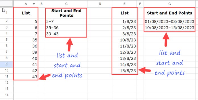
For example, if you consider the list {5, 6, 7, 35, 36, 39, 40, 41, 42, 43}, the start and end points will be the ranges 5–7, 35–36, and 39–43.

To generate this type of range, we may need to code a complex formula that is also easy to use.
Array Formula to Return Start and End Points from a List in Google Sheets
I have two formulas, one for numbers and the other for dates.
The formulas are almost the same. The only difference is the additional date formatting added to the formula that returns start and end points from a list of dates.
So, I’ll provide the formula for returning date ranges from a date list and highlight the part that you should remove when you use it with a numeric column.
Master Formula:
=ARRAYFORMULA(
     LET(
          list, E2:E,
          seq, SPLIT(FLATTEN(SPLIT(TEXTJOIN("|",TRUE,IFNA(
               XLOOKUP(
                    SEQUENCE(MAX(list)-MIN(list)+1,1,MIN(list)),
                    list,
                    list
               ),",")),",")),"|"),
          fltr, FILTER(seq,CHOOSECOLS(seq,1)<>"|"),
          BYROW(fltr,LAMBDA(r,
               TEXTJOIN("–",TRUE,TO_DATE(MIN(r)),IF(MAX(r)=MIN(r),,TO_DATE(MAX(r)))))
          )
     )
)
Yes, you need to remove the TO_DATE functions from the formula when you use it with a numeric list.
Other than that, you need to make only one change in the formula. That is to replace E2:E with the range that contains the list in your sheet.
If you are someone who is interested in learning advanced Google Sheets formulas, you may want to know how this formula returns multiple start and end points from a list in a single step.
I will explain that first. Then I will share with you how to use the returned result to count or sum the values in another column falling within this range.
Anatomy of the Formula
There are four key steps involved in the above formula. Here they are:

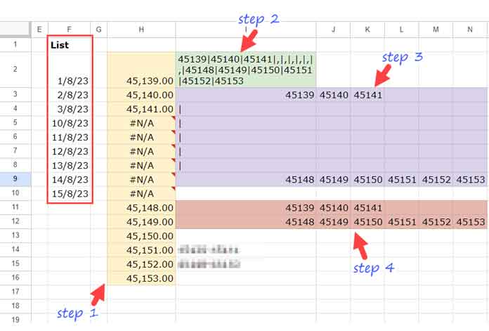
Step 1
The first step formula in cell H2 is an XLOOKUP array formula.
Formula:
=ARRAYFORMULA(XLOOKUP(SEQUENCE(MAX(F2:F)-MIN(F2:F)+1,1,MIN(F2:F)),F2:F,F2:F))Syntax:
XLOOKUP(search_key, lookup_range, result_range, [missing_value], [match_mode], [search_mode])Where:
- search_key: is
SEQUENCE(MAX(F2:F)-MIN(F2:F)+1,1,MIN(F2:F))which is the SEQUENCE populated using the MIN and MAX values in the list. - lookup_range: is
F2:F - result_range: is
F2:F
The formula matches the search keys in lookup_range and returns the matching values from the result_range. The purpose is to remove the missing values in the list from the sequence.
Note: The output will be date values if the list contains dates. That’s why we have used TO_DATE in our master formula to format them back to dates.
This is one of the main steps in returning start and end points from a list of dates or numbers in Google Sheets.
Step 2
Please see the first step result in the range H2:H16. The XLOOKUP function places #N/A wherever the sequence has gaps. In the next step, we will replace them with a comma and then TEXTJOIN all of the values. The delimiter will be a pipe.
Here is the second-step formula used in cell I2.
=ARRAYFORMULA(TEXTJOIN("|",TRUE,IFNA(H2:H,",")))Step 3
In the next step, we will SPLIT the above result twice and then FLATTEN it. I’ve placed the following formula in cell I3.
=ARRAYFORMULA(SPLIT(FLATTEN(SPLIT(I2,",")),"|"))Step 4
The next formula in cell I11 filters out the rows containing pipe in the first column.
=FILTER(I3:N9,I3:I9<>"|")Step 5 (Final)
We just need to extract the minimum and maximum values from each row of the step 4 result and join them with a dash.
We can use the following BYROW LHF for that.
=BYROW(I11:N12,LAMBDA(r,TEXTJOIN("-",TRUE,MIN(r),MAX(r))))This way, we can return the start and end points from a list of dates or numbers in Google Sheets.
Aggregate Data Corresponding to Generated Start and End Points from a List
At the very beginning of this tutorial, I explained the main purpose of returning start and end points from a list of numbers or dates in Google Sheets. It is to find the missing sequence values.
The other purpose is to summarize data based on the range returned by the formula. I will explain it with two examples. I am sure you will find it interesting.
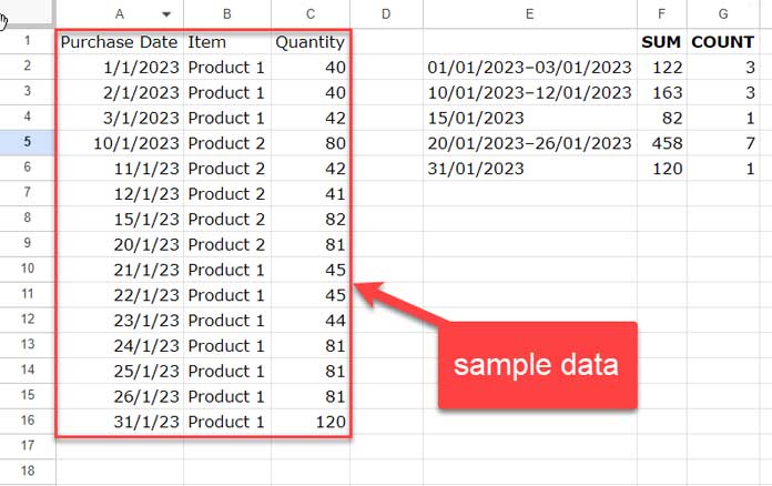
In the following example, we have purchase dates, items, and purchase quantities in the range A1:C.

Our formula in cell E2 returns the start and end date points from the list of dates (purchase dates) in the range A2:A. I am not repeating the formula, as you can simply replace E2:E in my master formula with A2:A.
Our focus is on the formulas in the columns F and G.
SUMIF Start and End Dates (Date Range) in Google Sheets
I have used the following SUMIF in cell F2 to sum values that fall between the start and end points, also known as the date range, in cell E2.
Syntax: SUMIF(range, criterion, [sum_range])
Formula:
=SUMIF(
     ISBETWEEN($A$2:$A,CHOOSECOLS(SPLIT(E2,"–"),1),CHOOSECOLS(SPLIT(E2,"–"),2)),
     TRUE,
     $C$2:$C
)
Where:
- range:
ISBETWEEN($A$2:$A,CHOOSECOLS(SPLIT(E2,"–"),1),CHOOSECOLS(SPLIT(E2,"–"),2)) - criterion:
TRUE - sum_range:
C$2:$C
I have copied and pasted this formula in cells F3 and F5.
The formula in cell F4 is =SUMIF($A$2:$A,E6,$C$2:$C), which I have also copied and pasted to cell F6.
Note: The delimiter in the SPLIT function is an en dash (–), not a hyphen (-).
COUNTIF Start and End Dates (Date Range) in Google Sheets
We can count the values corresponding to the returned start and end points from the purchase dates in range A2:A. For that, we can use the COUNTIF function.
Syntax:
COUNTIF(range, criterion)I have used the following COUNTIF formula in cell G2:
=COUNTIF(
     ISBETWEEN($A$2:$A,CHOOSECOLS(SPLIT(E2,"–"),1),CHOOSECOLS(SPLIT(E2,"–"),2)),
     TRUE
)
Where:
- range:
ISBETWEEN($A$2:$A,CHOOSECOLS(SPLIT(E2,"–"),1),CHOOSECOLS(SPLIT(E2,"–"),2)) - criterion:
TRUE
I have copied and pasted this formula into cells G3 and G5.
The COUNTIF formula in cell G4 is =COUNTIF(A2:A,E4), which I have also copied and pasted into cell G6.


