


")


")

")
")
 in Excel & Google Sheets")


In this post, let’s learn how to highlight adjacent duplicates in Google Sheets, including both row-wise and column-wise scenarios.
The conditional formatting for this is quite straightforward.
Sometimes, we may need to find duplicate values in consecutive cells—whether in rows or columns—not scattered across the sheet.
I’ve got conditional format rules that can help you identify such adjacent duplicates effectively.
For example, if we have the text “apple” in cells A2, A4, A5, and A7, the formula should highlight only A4 and A5—because those are the consecutive duplicates.
You can even choose whether to highlight both A4 and A5 or just A5 (i.e., from the second occurrence onward).
Let’s look at how to highlight adjacent duplicates in Google Sheets with a few simple formulas.
Using Conditional Formatting to Highlight Adjacent Duplicates (Row or Column-Wise)
In the first example, we’ll use a custom formula rule with conditional formatting to highlight all occurrences of consecutive duplicate values.
Later, we’ll see how to exclude the first occurrence.
Highlight All Consecutive Duplicate Values in Google Sheets
Let’s start with the column-wise data.
Column-Wise Data
You can use this LEN and logical AND based formula for data in the range B2:I2:
=AND(LEN(B2), B2=C2)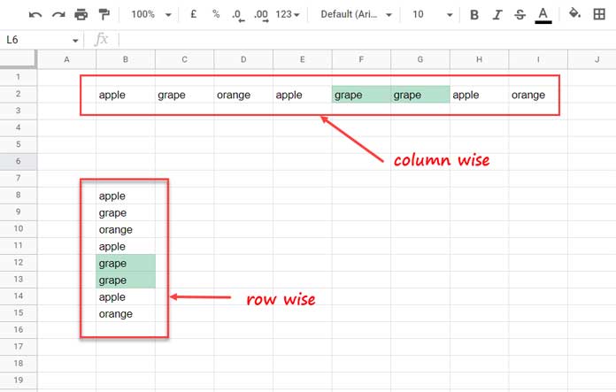
You’ll need to apply this formula twice—first for B2:I2 and then for C2:I2. Here’s how:
- Go to Format > Conditional formatting.
- In the sidebar, under Apply to range, enter
B2:I2. - Under Format rules, select Custom formula is and enter the formula:
=AND(LEN(B2), B2=C2) - Choose a fill color to highlight the adjacent duplicate values.
- Click Add another rule.
- Set Apply to range as
C2:I2and keep the same formula. - Click Done.
This will highlight all consecutive duplicate values in the row.
Note: To include more rows, such as B3:I3, simply update the ranges to B2:I3 and C2:I3.
Row-Wise Data
You can follow the same method to highlight adjacent duplicates in rows (i.e., vertical data).
Refer to the range B8:B15 in the earlier screenshot.
Use the following formula:
=AND(LEN(B8), B8=B9)Apply it twice—once for B8:B15 and then for B9:B15.
Note: If you have additional columns (like C8:C15), update the “Apply to range” to B8:C15 and B9:C15.
Highlight Adjacent Duplicates Except the First Occurrence
Now, let’s say you want to highlight only from the second occurrence onward—excluding the first of the adjacent duplicates.
To do that, simply delete one of the two rules we created earlier.
- For horizontal (row-wise) data: Delete the rule for
B2:I2. Keep only the one forC2:I2. - For vertical (column-wise) data: Delete the rule for
B8:B15. Keep only the one forB9:B15.
This way, only the second (or further) cells in an adjacent duplicate sequence get highlighted.
Here’s how the result will look:
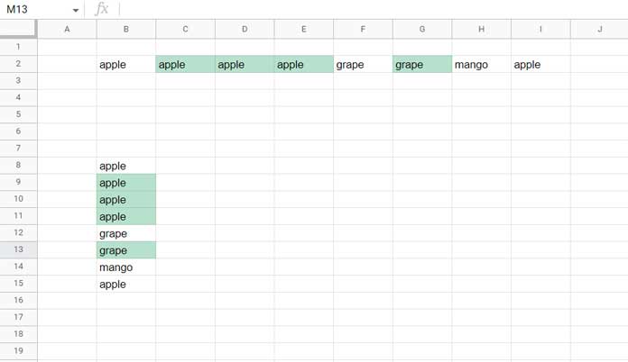
You can now clearly see the difference—consecutive duplicates are highlighted, except the first one in each group.
That’s how you can find and highlight adjacent duplicates in Google Sheets, whether row-wise or column-wise. Simple and effective!
Thanks for the read. Enjoy!