When you come across the concept of flipping values in a column or columns in Google Sheets, refrain from immediately assuming that it can be achieved through regular SORT or TRANSPOSE functions. So, what does flipping entail, and how can you reverse the values in a column?
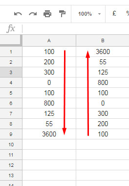
To comprehend the concept of flipping a column, refer to the image below.

I hope you can understand the concept of flipping numbers in a column in Google Sheets. Likewise, you can flip a column containing text strings. It’s important to note that flipping is distinct from normal sorting in descending or ascending order.
Flipping involves reversing the order of values in a column, placing the last row’s value in the first row, and so on. It’s distinct from regular sorting, which arranges values in ascending or descending order based on their content. Flipping maintains the original values themselves; it changes their relative positions within the column.
Additionally, the formula will vary depending on whether you want to include data in an infinite (opened) range (e.g., A2:A) or a finite (closed) range (e.g., A2:A10).
You may have come across solutions for flipping a column in Google Sheets, such as using a helper column with sequential numbers. Here is an example using the helper column approach.
Flip/Reverse a Column in Google Sheets – Helper Column Approach
How to Flip a Finite Column Range in Google Sheets
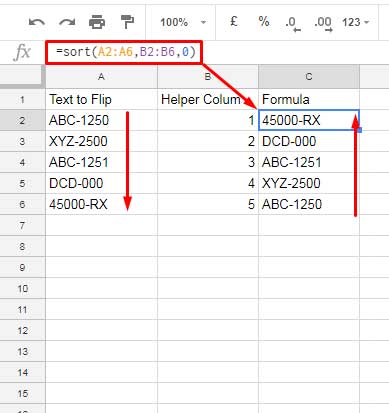
Here, I am flipping the values in column A to column C with the assistance of sequential numbers in the helper column B. Observe how the values are reversed in column C.

Undoubtedly, the SORT function plays a crucial role. Within the SORT function, we utilize an external column to sort our data, and that’s precisely what we are doing here. The relevant part of the function syntax is as follows:
SORT(range, sort_column, is_ascending)In this case, our external column (sort column) is the helper column B, and we need to sort the data in descending order based on this column. The formula looks like this:
=SORT(A2:A6, B2:B6, 0)Is it possible to use an infinite column range in this formula? Yes, it is. However, there are some changes to the formula, as outlined in the following section.
How to Flip an Infinite Column Range in Google Sheets
This time, I am omitting the screenshot. Once again, the values in column A remain the same, but I am adjusting the data range in the formula to encompass infinite rows. Here is the formula to flip an infinite column in Google Sheets:
=SORT(A2:A, B2:B, 0)Now, here is a crucial step:
Remove the values in the range B2:B. This entails eliminating the sequential numbers in the helper column.
You can employ one of the formulas below in cell B2, which automatically generates row numbers:
=ArrayFormula(IF(LEN(A2:A), ROW(A2:A),))
=ArrayFormula(ROW(A2:A) * N(A2:A<>""))
These formulas will populate column B with row numbers against all non-blank cells in column A. That concludes the helper column approach.
I understand that some of you desire a formula to flip a finite/infinite column range in Google Sheets without utilizing any helper column.
Flip a Column in Google Sheets – Non-Helper Column Approach
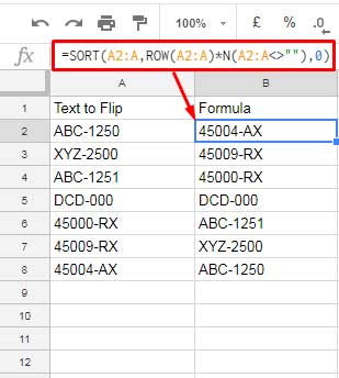
Here, there is no distinction between finite and infinite. The formula remains consistent:
=SORT(A2:A, ROW(A2:A)*N(A2:A<>""), 0)
In this, I’ve used the helper column formula within SORT to replace the helper column range. However, I’ve removed the ARRAYFORMULA function since it’s not required within SORT.
That’s it. I have presented all possible solutions for flipping a column in Google Sheets.
Can you flip multiple column ranges in Google Sheets using the above formula?
Yes, you can. The formula remains almost identical. Simply incorporate the additional columns in the SORT.
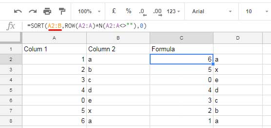
Consider an example where you have two columns (A2:B) to flip. In such a scenario, you can utilize this formula:
=SORT(A2:B, ROW(A2:A)*N(A2:A<>""), 0)
Normally, my tutorial contains the formula explanation part in most cases. With that, I intend to empower you to code complex formulas yourself.
Are you curious to know how this last formula works?
Formula Explanation:
Formula:
=SORT(A2:B, ROW(A2:A)*N(A2:A<>""), 0)Now I will explain the logic. Compare it to the formula below, where ROW(A2:A) replaces the ROW(A2:A)*N(A2:A<>""):
=SORT(A2:B, ROW(A2:A), 0)However, it has a problem. It assigns row numbers regardless of the values in column A.
For instance, if your column A has values only up to the 5th row, and your spreadsheet has 1000 rows, the ROW(A2:A) formula would still place numbers in all the rows (not physically). This creates issues when sorting in descending order.
Your flipped column would end up with numerous blank cells at the top. To address this, we need to use either the LEN function or the N function to limit the number of rows returned by the ROW function. In this case, the N function serves that purpose:
=ArrayFormula(ROW(A2:A) * N(A2:A<>""))Where:
ROW(A2:A)returns row numbers.N(A2:A<>"")returns 1 for non-blank cells and 0 for blank cells.
Simply enter this formula in cell D2, E2, or any second row. You will observe that this formula assigns row numbers up to the last non-blank cell in column A and fills the remaining cells with the value zero.


This doesn’t quite match your infinite column criteria, but for those with common, finite ranges to reverse, I think a better pattern is:
SORT(array,SEQUENCE(rows(array)),0).The benefit of this sorting, rather than using your ROWS()*N() method, is that it retains any blanks and preserves the same size and height of the original array or range. It simply reverses any 2D array it’s given, including spaces, blanks, BOOLEAN, or even errors in cells.
Hi,
I have some data in a row and want to flip it similarly. It is time-series data, and I want to use the sparkline function on it.
Can you help?
Hi, Abhinav Mehrotra,
Please check this guide – How to Reverse an Array in Google Sheets [Fixed and Dynamic Array]
If that doesn’t answer, please send a sample sheet via reply below.
Thanks. It works like a charm. I ran into the only issue that in 3 places it was Balancing – the formula is case sensitive. So, I had to correct those 3 entries. And yes, it is not equal to balancing.
Hi, SPH,
I am glad that I could help you.
Regarding the case sensitive issue, we can solve it using either of the LOWER or UPPER functions. In my example below, I am using the LOWER()
You can rewrite the
not(Col9)='balancing'part tonot(lower(Col9))='balancing'Hello,
How can I use this with FILTER? My filter string is
=filter(A2:S,C2:C"",I2:I"balancing")and I want to flip it. At present, there are 152 rows but these will keep increasing.
Thanks
Hi, SPH,
It seems my site’s EDITOR removed the comparison operators in your formula and I guess it’s “not equal to”.
The solution to your problem:
First, flip the table (columns) using my formula.
SORT(A2:S,ROW(A2:A)*N(not(A2:A="")),0)Then use QUERY to wrap it to filter the table.
Example:
=query(SORT(A2:S,ROW(A2:A)*N(not(A2:A="")),0),"Select * where Col3 is not null and not(Col9)='balancing'")Under “Flip a Column in Google Sheets – Non-Helper Column Approach” you put “Here there is no finite/infinite difference. The formula is the same!”
But it doesn’t seem to work for the finite case – it’s looking at the entire column, even if I want to restrict it to the first n rows.
If there are unrelated rows below the bottom-most element I want to consider, even if I leave a blank row, suddenly they appear as if they were part of the original list.
Hi, Michael,
I meant to say you can either use A2:A or A2:A100 if there are values in A2:A100. I forgot that some of you may want to flip part of the data in the column.
In the finite (closed range) case, the formula seems pretty simple.
To flip A2:A50, simply use the ROW function within SORT as the sort by.
=sort(A2:A50,row(A2:A50),0)To avoid blank rows in the range A2:A50, and reverse the data, you can use the below formula.
=SORT(A2:A50,ROW(A2:A50)*N(A2:A50<>""),0)I hope this helps?