


")


")

")
")
 in Excel & Google Sheets")


You can identify duplicates with the same date by highlighting or filtering the relevant values in Google Sheets. This technique is especially useful in real-world scenarios where the same item or action may occur more than once on the same day. For example:
- Detecting customers who placed multiple orders on the same day
- Tracking repeated entries of the same inventory item within a day
- Identifying duplicate logins or access events based on timestamps
- Filtering out repeated medical prescriptions issued to the same patient on a single date
In this tutorial, I’ll show you how to identify duplicates with the same date in Google Sheets using a dynamic formula. Whether your data includes just a timestamp and customer name or more fields like order ID or item details, this approach can adapt to your structure. It’s ideal for spotting repeated actions—like multiple orders by the same person on a single day—and can help you clean, filter, or highlight such duplicates for further analysis.
Sample Data
| Timestamp | Customer Name | Order ID |
| 01/04/2023 09:12:00 | Bianca | A001 |
| 01/04/2023 10:45:00 | Johnie | B001 |
| 01/04/2023 15:18:00 | Bianca | A002 |
| 02/04/2023 11:00:00 | Milo | C001 |
| 02/04/2023 13:22:00 | Bianca | A003 |
| 02/04/2023 16:00:00 | Milo | C002 |
| 03/04/2023 09:00:00 | Johnie | B002 |
| 03/04/2023 11:35:00 | Johnie | B003 |
In this data:
- Bianca placed two orders on April 1st
- Milo placed two orders on April 2nd
- Johnie placed two orders on April 3rd
These are the types of same-day duplicates you may want to filter or highlight.
Tip: If you want to isolate redundant records for deletion or flagging, use highlighting. If you’re reviewing true duplicates for analysis or cleanup, use filtering.
Filter Duplicates with Same Date in Google Sheets (Identifying True Duplicates)
To filter duplicates with the same date in Google Sheets, use this formula:
=ARRAYFORMULA(
  LET(
    data, A2:C,
    dtCol, A2:A,
    nameCol, B2:B,
    rc, COUNTIFS(nameCol, nameCol, INT(dtCol), INT(dtCol), ROW(dtCol), "<=" & ROW(dtCol)),
    ftrDt, FILTER(dtCol, rc > 1),
    ftrName, FILTER(nameCol, rc > 1),
    FILTER(data, XMATCH(INT(dtCol) & nameCol, INT(ftrDt) & ftrName))
  )
)
You can use this in datasets with either a date or timestamp column. The output will filter all entries with duplicate names on the same date:
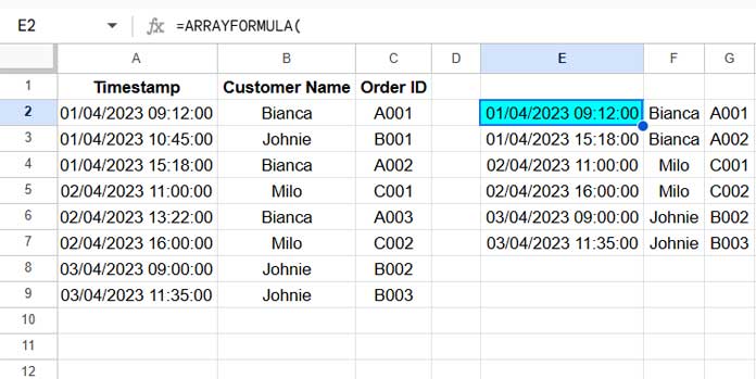
If a person placed multiple orders on the same day, all of those orders will be included in the filtered result.
Formula Explanation
data: Refers to the range A2:CdtCol: The timestamp/date column (A2:A)nameCol: The customer name column (B2:B)rc: A running count of each [name + date] pair usingCOUNTIFS, whereINT(dtCol)strips the time from the timestampftrDtandftrName: Filtered lists of dates and names with more than one occurrence- Final
FILTER: UsesXMATCHto return rows where the combination of date and name exists in the list of duplicates
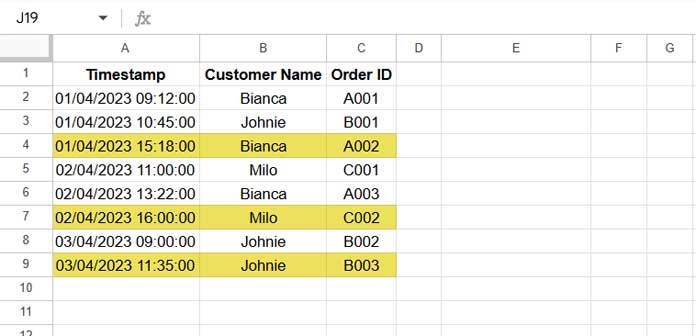
Highlight Duplicates with Same Date in Google Sheets (Isolating Repeats)
To highlight only the second occurrence and beyond (treating the first as original), follow these steps:
- Select range
A2:C - Go to Format > Conditional formatting
- Under Format rules, select Custom formula is
- Enter this formula:
=ARRAYFORMULA(
  LET(
    dtCol, $A$2:$A,
    nameCol, $B$2:$B,
    rc, COUNTIFS(nameCol, nameCol, INT(dtCol), INT(dtCol), ROW(dtCol), "<=" & ROW(dtCol)),
    ftrDt, FILTER(dtCol, rc > 1),
    ftrName, FILTER(nameCol, rc > 1),
    XMATCH($A2 & $B2, ftrDt & ftrName)
  )
)- Choose a highlight color and click Done
Highlight Rule Explanation
This formula mirrors the one used for filtering but is adapted for conditional formatting. It checks if the combination of date and name in a row exists among duplicates:
XMATCH($A2 & $B2, ftrDt & ftrName)If it does, the row is highlighted—starting from the second occurrence.
Related Resources
- Highlight Duplicates in Google Sheets
- Highlight Partial Matching Duplicates in Google Sheets
- Highlighting Visible Duplicates in Google Sheets
- Highlight Max Value Leaving Duplicates Row-Wise
- Highlight Duplicate Values Based on Occurrence Days
- How to Highlight Conditional Duplicates in Google Sheets
- How to Highlight Adjacent Duplicates in Google Sheets