To filter by month, you can use built-in filter tools such as the Data menu Filter and Slicer, or the FILTER and QUERY functions in Google Sheets.
I usually use the QUERY function to filter my data because I am very familiar with it. However, we can’t always depend on functions to filter data. Why?
The reason is that the functions extract the data into a new range. If you don’t want that, the options are the filter tools mentioned above.
The filter tools in Google Sheets are flexible, as they accept custom formulas similar to conditional formatting rules. You can use the same custom formulas when you filter your data using the Filter or Slicer, as well as the filtering applied when using the built-in tables.
In this tutorial, we will learn how to filter by month using the QUERY and FILTER functions and built-in tools in Google Sheets.
Filter by Month Using the Built-in Tools in Google Sheets
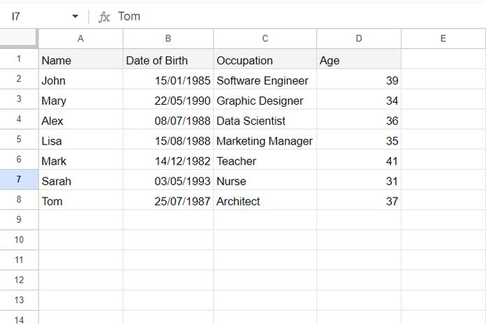
Let’s filter the sample data, which contains names in column A, their date of birth in column B, occupation in column C, and their age in column D.
A1, B1, C1, and D1 contain the field labels. We want to filter column B, and you should write the formula for cell B2.

Let me introduce the filter-by-month formulas for use with the Filter and Slicer tools first, and then we will move on to the filtering process.
Custom Formulas for Filtering
Month:
To filter column B for dates that fall in July, you can use the following formula:
=MONTH($B2)=7Data Falls Between Two Months:
To filter column B for dates that fall between July and August, use the following formula:
=AND(
   MONTH($B2)>=7,
   MONTH($B2)<=8
)
Month and Year:
If you want to filter by a specific month and year, for example, July 1988, the formula will be:
=EOMONTH($B2, -1)+1=DATE(1988, 7, 1)Explanation:
EOMONTH(B2, -1)+1converts the date in B2 to the start date of the month.DATE(1988, 7, 1)represents the filter criterion, with the syntaxDATE(year, month, day)for July 1988.
Data Falls Between Two Months in a Specific Year:
If your data spans more than one year, filtering data by month that falls across two months requires specifying both the month and year.
For example, to filter data that falls in July and August 1988, you can use the following formula:
=AND(
   $B2>=DATE(1988, 7, 1),
   $B2<=EOMONTH(DATE(1988, 8, 1), 0)
)
Explanation:
$B2>=DATE(1988, 7, 1)tests whether the date in B2 is greater than or equal to the beginning of July 1988.$B2<=EOMONTH(DATE(1988, 8, 1), 0)tests whether the date in B2 is less than or equal to the end of August 1988.
Filter Using the Filter Menu:
Assume you want to filter the people whose date of birth falls in the 7th month. Here’s how to filter the data:

- Select the data range, in this case, A1:D.
- Click Data > Create a filter.
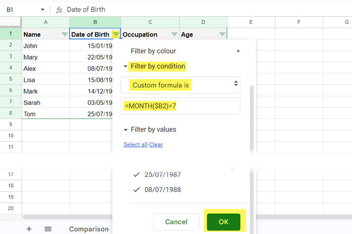
- Click on the filter drop-down in cell B1 and select Filter by condition.
- Choose Custom formula is from the options.
- Enter the formula:
=MONTH($B2)=7 - Click OK.
We have seen how to filter by month using the Filter tool in Google Sheets. I’ve provided some additional formulas above to specify year and month durations as well. You can similarly try those formulas.
Filter Using the Slicer Tool
Filtering by month using the Slicer tool is similar to the Filter tool.

If you prefer using the Slicer for filtering, follow these steps:
- Select the data range A1:D.
- Click Data > Add a Slicer.
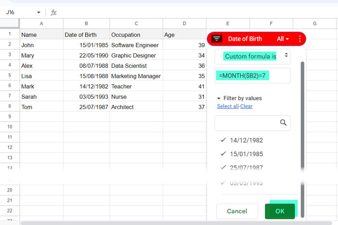
- In the Slicer sidebar panel, under Column, select the field label of the column to filter, in this case, Date of Birth.
- Click the Slicer drop-down and select Filter by condition.
- Choose Custom formula is.
- Enter the following formula in the field below:
=MONTH($B2)=7 - Click OK.
Similarly, try using the other provided custom formulas to include year or month ranges in your filtering.
Filter by Month Using Functions in Google Sheets
If you prefer to extract the data to a new range instead of filtering the source, consider the following formulas.
The following FILTER formulas filter the data for the month of July (month number 7):
Without year:
=FILTER(A1:D, MONTH(B1:B)=7)With year:
=FILTER(A1:D, EOMONTH(B1:B, -1)+1=DATE(1988, 7, 1))To filter data that falls between two months, for example, July and August, use the following:
Without year:
=FILTER(A1:D, MONTH(B1:B)>=7, MONTH(B1:B)<=8)With year:
=FILTER(A1:D, B1:B>=DATE(1988, 7, 1), B1:B<EOMONTH(DATE(1988, 8, 1), 0))For those who wish to use QUERY, here are the formulas:
Filter by Month:
=QUERY(A:D, "SELECT * WHERE MONTH(B)=6", 1)Note: In QUERY, the month numbers range from 0 to 11, where 0 represents January and 11 represents December.
Between Two Months:
=QUERY(A:D, "SELECT * WHERE MONTH(B)>=6 AND MONTH(B)<=7", 1)


