Google Forms responses in a connected sheet contain a timestamp column. Additionally, some users utilize Google Apps Script (GAS) to input timestamps for their data. However, I am not discussing that here. Instead, I will explain how to compare a timestamp with a standard date in Google Sheets, as one represents a pure date while the other includes time. Consequently, the values differ significantly for a logical IF test.
For example, a timestamp like “31/12/2017 20:46:10” is not equal to “31/12/2017.” Therefore, a logical test may yield unexpected results if you simply evaluate two dates.
When performing a logical test in a cell or array that contains timestamps, it is essential to know how to remove the time component from a timestamp. This allows you to use the cleaned date within your logical test.
There are various methods to extract the date from timestamps and return only the date. I have already detailed these methods in the tutorial: Extracting Date From Timestamp in Google Sheets: 5 Methods.
I hope you have reviewed the tutorial mentioned above. Now, let’s return to our topic and example.
Examples
Here are two basic logical tests that will help you understand the correct way to compare a timestamp with a standard date in Google Sheets.
Cell A3 contains the datetime 30/09/2024 22:10:15, and cell B3 contains the date 30/09/2024. One is a datetime, and the other is a date. The following formula in cell C3 would return TRUE:
=A3>B3This is because the datetime in A3 is greater than the date in B3, even though both fall on the same day, i.e., 30/09/2024.
If you want to extract the date from A3 and compare it to the date in B3, you may use the following formula:
=INT(A3)>B3This would return FALSE since both dates are the same.
Comparing Timestamps in a Column with a Standard Date
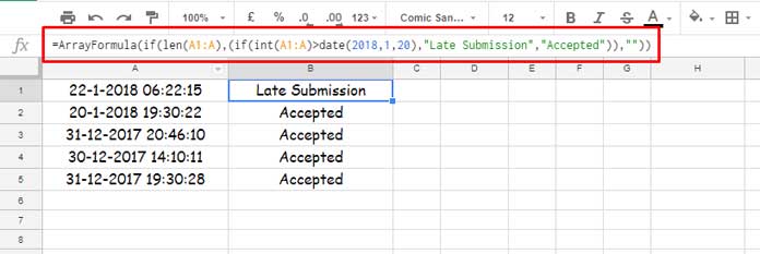
In the following example, we will test the timestamps in column A against a standard date using IF logical tests in two ways: one with the actual datetime in column A and another after removing the time component. Then, we will observe the difference.
The logical test is as follows:
If the date in column A is greater than “20-01-2018,” the formula should return “Late Submission”; otherwise, it should return “Accepted.”

Now, I would like to draw your attention to the two array formulas below. The first one is the original formula I’ve used to compare the timestamp with the standard date in Google Sheets. Refer to the formula in the above screenshot.
Formula 1 (in cell B1):
=ARRAYFORMULA(
   IF(
      LEN(A1:A),
      IF(INT(A1:A) > DATE(2024, 9, 30), "Late Submission", "Accepted"),
      ""
   )
)
In this formula, I’ve converted the timestamps in column A to standard dates using the INT function.
Note: The hardcoded date in the formula follows the DATE function syntax: DATE(year, month, day).
If you use the formula below, which is a standard logical test, it will return an incorrect result in row 2, as it treats the timestamp “20/01/2018 19:30:22” in row 2 and the date “20/01/2018” as two different values.
Formula 2:
=ARRAYFORMULA(
   IF(
      LEN(A1:A),
      IF(A1:A > DATE(2018, 1, 20), "Late Submission", "Accepted"),
      ""
   )
)
This illustrates how you can compare timestamps with a standard date in Google Sheets.
Resources
- Convert Unix Timestamp to Local DateTime and Vice Versa in Google Sheets
- Extract the Earliest or Latest Record in Each Category Based on Timestamp
- How to Convert a Timestamp to Milliseconds in Google Sheets
- How to Filter Timestamp in Query in Google Sheets
- How to Hardcode DATETIME Criteria within FILTER Function in Google Sheets
- How to Increment DateTime by One Hour in Google Sheets (Array Formula)
- How to Insert a Static Timestamp in Google Sheets
- How to Remove Milliseconds from Timestamps in Google Sheets
- How to Unique Rows Ignoring Timestamp Column in Google Sheets
- How to Use DateTime in Query in Google Sheets
- How to Use Timestamp within IF Logical Function in Google Sheets
- Vlookup Date in Timestamp Column in Google Sheets


