Highlighting the median in Google Sheets is simple when the median exists in your dataset. But when your list has an even number of values, the median is just the average of the two middle numbers — and that value might not be in the list at all.

That’s why the basic formula:

=A1=MEDIAN($A$1:$A)

…will fail silently in some cases.

In this guide, you’ll learn how to highlight the median in Google Sheets — even when it isn’t in the list — using a single Conditional Formatting formula that works for odd and even lists, and for both 1D and 2D ranges.

Why Highlight the Median in Google Sheets Matters

The median is a key measure of central tendency that’s often more representative than the average, especially when your data has outliers.

Highlighting the median in Google Sheets can help you:

• Spot the central value(s) quickly.
• Visualize data balance in reports or dashboards.
• Compare medians across datasets for trend analysis.

The Problem with Highlighting the Median in Even-Numbered Lists in Google Sheets

Consider these two lists:

Even list:

1  
2  
3  
4

The median is 2.5, which isn’t in the list.

Odd list:

1  
2  
3  
4  
5

The median is 3, which is in the list.

Since the median might not exist as an actual value in the even-numbered case, a direct median comparison can’t highlight it. You need a formula that finds the two middle values instead.

Formula to Highlight the Median in Google Sheets for Any Dataset

Here’s the universal formula you can use inside Conditional Formatting:

=XMATCH(
  range_start,
  LET(
    r, TOCOL(range, 3),
    mn, MEDIAN(r),
    xl, XLOOKUP(mn, r, r, ,-1),
    UNIQUE(VSTACK(xl, XLOOKUP(mn, r, r, ,1)))
  )
)

Where:

• range_start → the first cell in your selection (top-left if 2D).
• range → the full range to check (absolute references like $A$2:$C$10).

This method works whether your dataset is a single column, multiple columns, odd-sized, or even-sized.

Highlight the Median in a Single Column in Google Sheets

Dataset in B2:B:

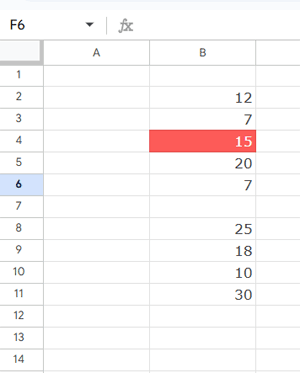
1. Select the range B2:B.
2. Go to Format → Conditional formatting.
3. Under Format cells if, choose Custom formula is.
4. Enter the following formula:

=XMATCH(
  B2,
  LET(
    r, TOCOL($B$2:$B, 3),
    mn, MEDIAN(r),
    xl, XLOOKUP(mn, r, r, ,-1),
    UNIQUE(VSTACK(xl, XLOOKUP(mn, r, r, ,1)))
  )
)

5. Pick a highlight color.
6. Click Done.

The median value (or both middle values if the median isn’t in the list) will now be highlighted.

Highlight the Median in Multiple Columns in Google Sheets

Dataset in A2:C:

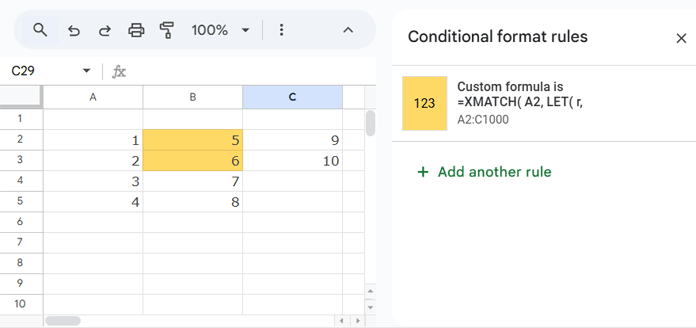
Formula for Conditional Formatting:

=XMATCH(
  A2,
  LET(
    r, TOCOL($A$2:$C, 3),
    mn, MEDIAN(r),
    xl, XLOOKUP(mn, r, r, ,-1),
    UNIQUE(VSTACK(xl, XLOOKUP(mn, r, r, ,1)))
  )
)

This formula flattens the entire range into a single column, calculates the median, and highlights either:

• the exact median (if it exists), or
• the two middle values (if it doesn’t).

How the Google Sheets Median Highlight Formula Works

Let’s break it down:

• TOCOL(range, 3) → Flattens your range into one column, ignoring blanks.
• MEDIAN(r) → Finds the median of the flattened list.
• First XLOOKUP → Looks for an exact match to the median, or the largest value ≤ median.
• Second XLOOKUP → Finds the exact match to the median, or the smallest value ≥ median.
• VSTACK + UNIQUE → Combines both results and removes duplicates.
• XMATCH → Checks if the current cell’s value is one of those middle values.

Why Does the Median Highlight Include Duplicates?

When the median value appears multiple times in your dataset, this formula will highlight all occurrences of that value. This helps you quickly spot every instance of the median, which is useful for identifying patterns or repeated central values.

In many cases, highlighting all duplicates of the median is actually a good thing. It shows the full picture rather than just one occurrence.

How to Override Highlighting for Duplicate Median Values

If you prefer to highlight only the first occurrence of the median value and ignore the rest, you can add an extra rule to your Conditional Formatting using COUNTIF.

For example, to exclude duplicates after the first occurrence in column A (for a range like A2:A or a multi-column range like A2:C), use this formula:

=COUNTIF($A$2:A2, A2)=1

This formula returns TRUE only for the first time a value appears in the range and FALSE for any duplicates below it.

Steps to Apply This Duplicate-Override Rule

• Select cell A2, then go to Format > Conditional formatting.
• Click on the existing rule to open it in the sidebar panel.
• At the bottom, click on “+ Add another rule”.
• In the new rule, enter the above COUNTIF formula as the custom formula.
• Set the fill color to white (or your spreadsheet’s background color) to effectively hide duplicates.
• Click Done.
• Finally, drag this new rule above the earlier median highlighting rule to ensure it applies first.

Why This Median Highlight Method Is the Best for Google Sheets

• Works for odd and even datasets.
• Handles single and multi-column ranges.
• Ignores blanks automatically.
• No scripts or helper columns required.

Related Tutorials

• MEDIAN Function in Google Sheets
• Item Wise Median Using Pivot Table in Google Sheets
• Percentile Rank Wise Conditional Formatting in Google Sheets
• Nested XLOOKUP Function in Google Sheets