To highlight the max value while leaving duplicates row-wise in Google Sheets, you can use a combination of the AND, RANK, UNIQUE, and COUNTIF functions.

You can use the MAX function to extract the max value in a row. When you want to find it in each row, you can use the BYROW lambda with MAX. However, instead of extracting the value, you might want to quickly visualize the max value in each row. This is where conditional formatting becomes useful.

Real-Life Example: Employee Sales Performance

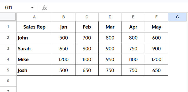
Consider a scenario where each row represents sales figures for different employees. Their sales amounts are spread across columns, where each column represents a different month.

You can apply a highlight rule to emphasize the max sale of each employee in their records. If an employee has the same max sale in multiple months, you may want to highlight only one occurrence to avoid clutter.

If that is the case, use the following formula to highlight the max value while leaving duplicates row-wise in Google Sheets:

=AND(RANK(A1, UNIQUE($A1:$Z1, TRUE))=1, COUNTIF($A1:A1, A1)<2)

Replace A1 with the first cell in the row, $A1:$Z1 with the reference to the entire row, and $A1:A1 with the first cell reference as a range.

You can replace RANK with MAX, but using RANK makes the formula more flexible. You can use it to highlight the first, second, and third largest unique values with different colors, which we will discuss later.

Highlighting Max Value While Leaving Duplicates in Row-Wise – Example

Sample Sales Data

Steps to Highlight the Max Value While Leaving Duplicates in Each Row

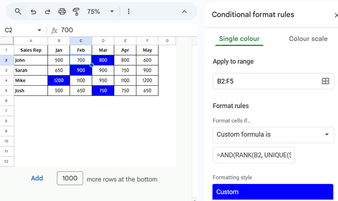
1. Select the range to highlight (e.g., B2:F5).
2. Click Format > Conditional Formatting.
3. Under Format rules, select Custom Formula Is.
4. Enter the following formula:=AND(RANK(B2, UNIQUE($B2:$F2, TRUE))=1, COUNTIF($B2:B2, B2)<2)
5. Choose a fill color (e.g., Blue).
6. Click Done.

This will highlight the max value while leaving duplicates unhighlighted in each row.

Formula Explanation

The formula used is:

=AND(RANK(B2, UNIQUE($B2:$F2, TRUE))=1, COUNTIF($B2:B2, B2)<2)

• RANK(B2, UNIQUE($B2:$F2, TRUE))=1 – Returns TRUE if the rank of B2 in the unique row range is equal to 1.
• COUNTIF($B2:B2, B2)<2 – Ensures that the value in B2 appears only once up to that point in the row, avoiding duplicate highlights.
• The AND function ensures that both conditions are met before highlighting the cell.

The RANK test applies to each value in the row with the row range, and the COUNTIF test applies to each value dynamically as it progresses through the row.

Proper use of relative and absolute cell references is crucial for correctly highlighting the max value while leaving duplicates row-wise in Google Sheets.

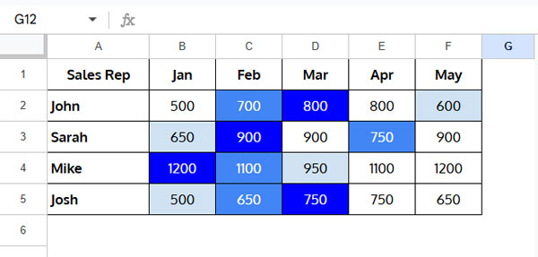
Highlight the Second and Third Largest Values While Leaving Duplicates in Each Row

To highlight the second largest value while leaving duplicates, modify the formula by replacing =1 with =2:

=AND(RANK(B2, UNIQUE($B2:$F2, TRUE))=2, COUNTIF($B2:B2, B2)<2)

For the third largest value, replace =1 with =3:

=AND(RANK(B2, UNIQUE($B2:$F2, TRUE))=3, COUNTIF($B2:B2, B2)<2)

Apply each rule separately, using different fill colors (e.g., Blue, Light Blue, and Grey) to make them stand out.

Related Resources

• How to Highlight the Largest 3 Values in Each Row in Google Sheets – Discusses various tie-breaking methods.
• Highlight Unique Top N Values in Google Sheets – Covers unique value highlighting in both rows and columns.
• Highlight Top 10 Ranks in Single or Each Column in Google Sheets – Focuses on rank-based highlighting.

By following these steps, you can effectively highlight the max value while leaving duplicates row-wise in Google Sheets, ensuring a clear and clutter-free visual representation of important data.